From the solar wind to the ground#
Abstract: We demonstrate a basic analysis of a geomagnetic storm using hapiclient & viresclient to access data from the solar wind (OMNI IMF), Low Earth Orbit (Swarm-derived auroral electrojet estimates), and the ground (INTERMAGNET observatory magnetic measurements).
%load_ext watermark
%watermark -i -v -p viresclient,hapiclient,pandas,xarray,matplotlib
Python implementation: CPython
Python version       : 3.11.6
IPython version      : 8.18.0

viresclient: 0.15.0
hapiclient : 0.2.6
pandas     : 2.1.3
xarray     : 2023.12.0
matplotlib : 3.8.2
Packages to use#
hapiclientto access solar wind data from OMNI (alternatively we could usepysat)For more examples with hapiclient, take a look at the demonstration notebooks
viresclientto access AEJs from Swarm, and B-field from ground observatoriesxarrayandmatplotlibfor data wrangling and plottingSee the xarray tutorial website to learn more
from copy import deepcopy
import numpy as np
import pandas as pd
import xarray as xr
import matplotlib.pyplot as plt

from viresclient import SwarmRequest
from hapiclient import hapi, hapitime2datetime
Time selection#
Let’s choose an interesting time period to study - the “St. Patrick’s day storm” of 17th March 2015. You can look at the wider context of this event using the interactive Space Weather Data Portal from the University of Colorado
We will use the same time window to fetch data from the different sources:
START_TIME = "2015-03-15T00:00:00Z"
END_TIME = "2015-03-20T00:00:00Z"
Solar wind data (OMNI)#
HAPI is an access protocol supported by a wide array of heliophysics datasets. We can use the Python package “hapiclient” to retrieve data from HAPI servers. In this case we will access the OMNI HRO2 dataset which provides consolidated solar wind data, and then we will show how we can load these data into pandas and xarray objects.
OMNI Combined, Definitive 1-minute IMF and Definitive Plasma Data Time-Shifted to the Nose of the Earth’s Bow Shock, plus Magnetic Indices - J.H. King, N. Papatashvilli (AdnetSystems, NASA GSFC)
To generate code snippets to use, and to see what data are available:
http://hapi-server.org/servers/#server=CDAWeb&dataset=OMNI_HRO2_1MIN¶meters=flow_speed&start=2000-01-01T00:00:00Z&stop=2000-02-01T00:00:00Z&return=script&format=python
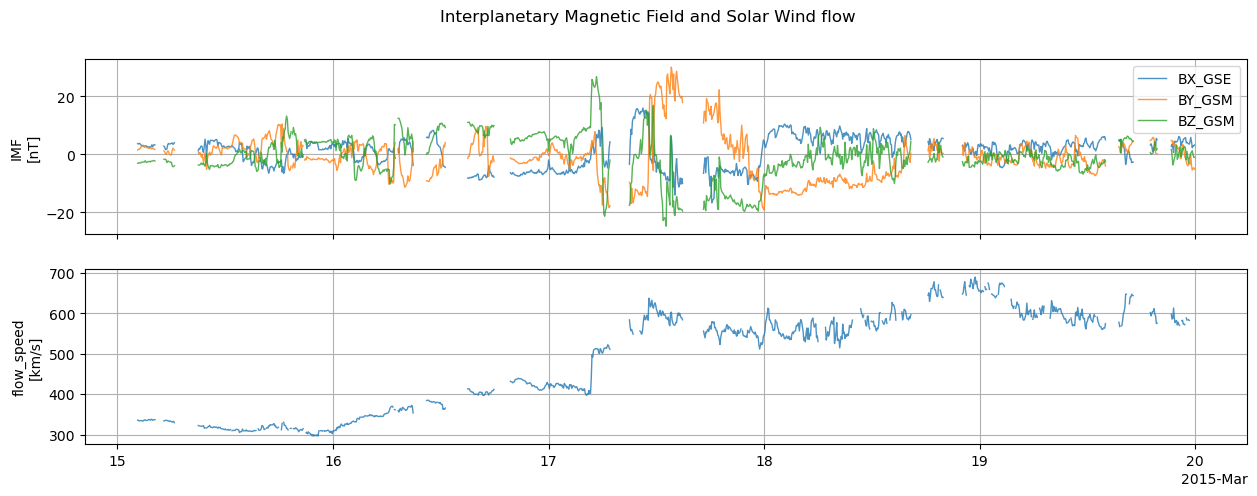
Here we will access five-minute-resolution measurements of the Interplanetary Magnetic Field (IMF) vector and the bulk flow speed of the solar wind:
def fetch_omni_data(start, stop):
    server = "https://cdaweb.gsfc.nasa.gov/hapi"
    dataset = "OMNI_HRO2_5MIN"
    parameters = "BX_GSE,BY_GSM,BZ_GSM,flow_speed"
    data, meta = hapi(server, dataset, parameters, start, stop)
    return data, meta


data, meta = fetch_omni_data(START_TIME, END_TIME)
Data are automatically loaded as a NumPy structured array and metadata as a dictionary:
data
array([(b'2015-03-15T00:00:00.000Z', 9.99999000e+03,  9.99999000e+03,  9.99999000e+03, 99999.9),
       (b'2015-03-15T00:05:00.000Z', 9.99999000e+03,  9.99999000e+03,  9.99999000e+03, 99999.9),
       (b'2015-03-15T00:10:00.000Z', 9.99999000e+03,  9.99999000e+03,  9.99999000e+03, 99999.9),
       ...,
       (b'2015-03-19T23:45:00.000Z', 3.03999996e+00, -4.92000008e+00, -5.99999987e-02, 99999.9),
       (b'2015-03-19T23:50:00.000Z', 2.91000009e+00, -4.63999987e+00, -1.02999997e+00, 99999.9),
       (b'2015-03-19T23:55:00.000Z', 3.20000005e+00, -5.13999987e+00, -1.04999995e+00, 99999.9)],
      dtype=[('Time', 'S24'), ('BX_GSE', '<f8'), ('BY_GSM', '<f8'), ('BZ_GSM', '<f8'), ('flow_speed', '<f8')])
meta
{'HAPI': '2.0',
 'resourceURL': 'https://cdaweb.gsfc.nasa.gov/misc/NotesO.html#OMNI_HRO2_5MIN',
 'contact': 'J.H. King, N. Papatashvilli @ AdnetSystems, NASA GSFC',
 'parameters': [{'name': 'Time',
   'length': 24,
   'units': 'UTC',
   'type': 'isotime',
   'fill': None},
  {'name': 'BX_GSE',
   'description': 'Bx (nT), GSE',
   'units': 'nT',
   'type': 'double',
   'fill': '9999.99'},
  {'name': 'BY_GSM',
   'description': 'By (nT), GSM, determined from post-shift GSE components',
   'units': 'nT',
   'type': 'double',
   'fill': '9999.99'},
  {'name': 'BZ_GSM',
   'description': 'Bz (nT), GSM, determined from post-shift GSE components',
   'units': 'nT',
   'type': 'double',
   'fill': '9999.99'},
  {'name': 'flow_speed',
   'description': 'Flow Speed (km/s), GSE',
   'units': 'km/s',
   'type': 'double',
   'fill': '99999.9'}],
 'startDate': '1995-01-01T00:00:00Z',
 'stopDate': '2026-01-31T23:55:00Z',
 'status': {'code': 1200, 'message': 'OK'},
 'x_server': 'https://cdaweb.gsfc.nasa.gov/hapi',
 'x_dataset': 'OMNI_HRO2_5MIN',
 'x_parameters': 'BX_GSE,BY_GSM,BZ_GSM,flow_speed',
 'x_time.min': '2015-03-15T00:00:00Z',
 'x_time.max': '2015-03-20T00:00:00Z',
 'x_requestDate': '2026-03-04T11:46:29',
 'x_cacheDir': '/tmp/hapi-data/cdaweb.gsfc.nasa.gov_hapi',
 'x_downloadTime': 4.547593593597412,
 'x_readTime': 0.00037169456481933594,
 'x_metaFileParsed': '/tmp/hapi-data/cdaweb.gsfc.nasa.gov_hapi/OMNI_HRO2_5MIN___.pkl',
 'x_dataFileParsed': '/tmp/hapi-data/cdaweb.gsfc.nasa.gov_hapi/OMNI_HRO2_5MIN_BX_GSE,BY_GSM,BZ_GSM,flow_speed_20150315T000000_20150320T000000.npy',
 'x_metaFile': '/tmp/hapi-data/cdaweb.gsfc.nasa.gov_hapi/OMNI_HRO2_5MIN___.json',
 'x_dataFile': '/tmp/hapi-data/cdaweb.gsfc.nasa.gov_hapi/OMNI_HRO2_5MIN_BX_GSE,BY_GSM,BZ_GSM,flow_speed_20150315T000000_20150320T000000.bin',
 'x_totalTime': 4.820730924606323}
We are now able to extract an array for a particular value like data["BZ_GSM"], and use the metadata to get full descriptions and units for the chosen parameter.
The metadata sometimes contains fill values used during data gaps (e.g. the 9999… values appearing above). Let’s use those to replace the gaps with NaN values:
def fill2nan(hapidata_in, hapimeta):
    """Replace bad values (fill values given in metadata) with NaN"""
    hapidata = deepcopy(hapidata_in)
    # HAPI returns metadata for parameters as a list of dictionaries
    # - Loop through them
    for metavar in hapimeta["parameters"]:
        varname = metavar["name"]
        fillvalstr = metavar["fill"]
        if fillvalstr is None:
            continue
        vardata = hapidata[varname]
        mask = vardata == float(fillvalstr)
        nbad = np.count_nonzero(mask)
        print("{}: {} fills NaNd".format(varname, nbad))
        vardata[mask] = np.nan
    return hapidata, hapimeta


data, meta = fill2nan(data, meta)
data
BX_GSE: 297 fills NaNd
BY_GSM: 297 fills NaNd
BZ_GSM: 297 fills NaNd
flow_speed: 401 fills NaNd
array([(b'2015-03-15T00:00:00.000Z',        nan,         nan,         nan, nan),
       (b'2015-03-15T00:05:00.000Z',        nan,         nan,         nan, nan),
       (b'2015-03-15T00:10:00.000Z',        nan,         nan,         nan, nan),
       ...,
       (b'2015-03-19T23:45:00.000Z', 3.03999996, -4.92000008, -0.06      , nan),
       (b'2015-03-19T23:50:00.000Z', 2.91000009, -4.63999987, -1.02999997, nan),
       (b'2015-03-19T23:55:00.000Z', 3.20000005, -5.13999987, -1.04999995, nan)],
      dtype=[('Time', 'S24'), ('BX_GSE', '<f8'), ('BY_GSM', '<f8'), ('BZ_GSM', '<f8'), ('flow_speed', '<f8')])
We can load the data into a pandas DataFrame to more readily use for analysis:
def to_pandas(hapidata):
    df = pd.DataFrame(
        columns=hapidata.dtype.names,
        data=hapidata,
    ).set_index("Time")
    # Convert from hapitime to Python datetime
    df.index = hapitime2datetime(df.index.values.astype(str))
    # df.index = pd.DatetimeIndex(df.index.values.astype(str))
    # Remove timezone awareness
    df.index = df.index.tz_convert("UTC").tz_convert(None)
    # Rename to Timestamp to match viresclient
    df.index.name = "Timestamp"
    return df


df = to_pandas(data)
df
/opt/conda/lib/python3.11/site-packages/hapiclient/hapitime.py:284: UserWarning: The argument 'infer_datetime_format' is deprecated and will be removed in a future version. A strict version of it is now the default, see https://pandas.pydata.org/pdeps/0004-consistent-to-datetime-parsing.html. You can safely remove this argument.
  Time = pandas.to_datetime(Time, infer_datetime_format=True).tz_convert(tzinfo).to_pydatetime()
| BX_GSE | BY_GSM | BZ_GSM | flow_speed | |
|---|---|---|---|---|
| Timestamp | ||||
| 2015-03-15 00:00:00 | NaN | NaN | NaN | NaN |
| 2015-03-15 00:05:00 | NaN | NaN | NaN | NaN |
| 2015-03-15 00:10:00 | NaN | NaN | NaN | NaN |
| 2015-03-15 00:15:00 | NaN | NaN | NaN | NaN |
| 2015-03-15 00:20:00 | NaN | NaN | NaN | NaN |
| ... | ... | ... | ... | ... |
| 2015-03-19 23:35:00 | 4.30 | -3.83 | 0.61 | NaN |
| 2015-03-19 23:40:00 | 2.26 | -5.46 | 1.24 | NaN |
| 2015-03-19 23:45:00 | 3.04 | -4.92 | -0.06 | NaN |
| 2015-03-19 23:50:00 | 2.91 | -4.64 | -1.03 | NaN |
| 2015-03-19 23:55:00 | 3.20 | -5.14 | -1.05 | NaN |
1440 rows × 4 columns
How can we get the extra information like the units from the metadata? Let’s construct dictionaries, units and description, that allow easier access to these:
def get_units_description(meta):
    units = {}
    description = {}
    for paramdict in meta["parameters"]:
        units[paramdict["name"]] = paramdict.get("units", None)
        description[paramdict["name"]] = paramdict.get("description", None)
    return units, description


units, description = get_units_description(meta)
units, description
({'Time': 'UTC',
  'BX_GSE': 'nT',
  'BY_GSM': 'nT',
  'BZ_GSM': 'nT',
  'flow_speed': 'km/s'},
 {'Time': None,
  'BX_GSE': 'Bx (nT), GSE',
  'BY_GSM': 'By (nT), GSM, determined from post-shift GSE components',
  'BZ_GSM': 'Bz (nT), GSM, determined from post-shift GSE components',
  'flow_speed': 'Flow Speed (km/s), GSE'})
The xarray.Dataset object has advantages for handling multi-dimensional data and for attaching of metadata like units. Let’s convert the data to an xarray.Dataset:
def to_xarray(hapidata, hapimeta):
    # Here we will conveniently re-use the pandas function we just built,
    # and use the pandas API to build the xarray Dataset.
    # NB: if performance is important, it's better to build the Dataset directly
    ds = to_pandas(hapidata).to_xarray()
    units, description = get_units_description(hapimeta)
    for param in ds:
        ds[param].attrs = {"units": units[param], "description": description[param]}
    return ds


ds_sw = to_xarray(data, meta)
ds_sw
/opt/conda/lib/python3.11/site-packages/hapiclient/hapitime.py:284: UserWarning: The argument 'infer_datetime_format' is deprecated and will be removed in a future version. A strict version of it is now the default, see https://pandas.pydata.org/pdeps/0004-consistent-to-datetime-parsing.html. You can safely remove this argument.
  Time = pandas.to_datetime(Time, infer_datetime_format=True).tz_convert(tzinfo).to_pydatetime()
<xarray.Dataset>
Dimensions:     (Timestamp: 1440)
Coordinates:
  * Timestamp   (Timestamp) datetime64[ns] 2015-03-15 ... 2015-03-19T23:55:00
Data variables:
    BX_GSE      (Timestamp) float64 nan nan nan nan nan ... 2.26 3.04 2.91 3.2
    BY_GSM      (Timestamp) float64 nan nan nan nan ... -5.46 -4.92 -4.64 -5.14
    BZ_GSM      (Timestamp) float64 nan nan nan nan ... 1.24 -0.06 -1.03 -1.05
flow_speed (Timestamp) float64 nan nan nan nan nan ... nan nan nan nan nanNow let’s plot these data:
def plot_solar_wind(ds_sw):
    fig, axes = plt.subplots(nrows=2, ncols=1, sharex=True, figsize=(15, 5))
    for IMF_var in ["BX_GSE", "BY_GSM", "BZ_GSM"]:
        ds_sw[IMF_var].plot.line(
            x="Timestamp", linewidth=1, alpha=0.8, ax=axes[0], label=IMF_var
        )
    axes[0].legend()
    axes[0].set_ylabel("IMF\n[nT]")
    axes[0].set_xlabel("")
    ds_sw["flow_speed"].plot.line(x="Timestamp", linewidth=1, alpha=0.8, ax=axes[1])
    axes[1].set_ylabel("flow_speed\n[km/s]")
    axes[1].set_xlabel("")
    axes[0].grid()
    axes[1].grid()
    fig.suptitle("Interplanetary Magnetic Field and Solar Wind flow")
    return fig, axes


fig_sw, axes_sw = plot_solar_wind(ds_sw)

Auroral electrojets as measured by Swarm#
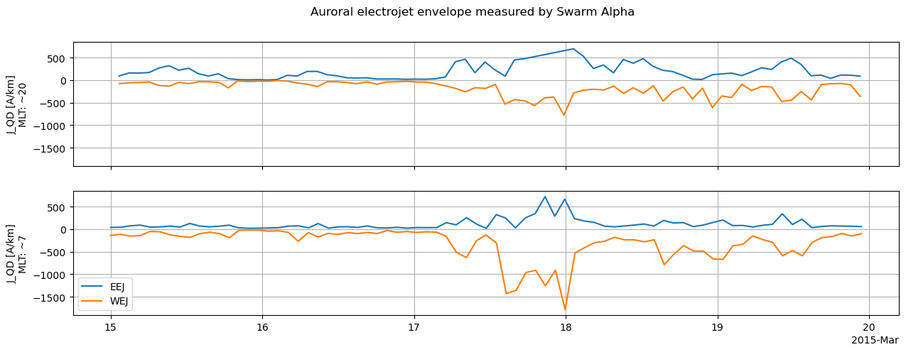
Since spacecraft move, it is difficult to extract a simple time series that can be easily tracked. From the complex Swarm product portfolio, we will pick a particular derived parameter: the peak auroral electrojet intensities derived from each pass over the current system. This signal tracks reasonably well from one orbit to the next (when separated into four orbital segments - accounting for two passes over the auroral oval in different local time sectors, and over the northern and southern hemispheres).
To keep things a bit simpler, we will retrieve data only from Swarm Alpha over the Northern Hemisphere. The auroral electrojet peaks and boundaries for Swarm Alpha are contained within the product named SW_OPER_AEJAPBL_2F. Here is how we can access these data:
def fetch_Swarm_AEJ(start_time, end_time):
    request = SwarmRequest()
    # Meaning of AEJAPBL: (AEJ) Auroral electrojets
    #                     (A)   Swarm Alpha
    #                     (PBL) Peaks and boundaries from LC method
    # J_QD is the current intensity along QD-latitude contours
    # QDOrbitDirection is a flag (1, -1) marking the direction of the
    #   satellite (ascending, descending) relative to the QD pole
    # MLT is magnetic local time, evaluated according to the
    #   quasi-dipole magnetic longitude and the sub-solar point
    #   (see doi.org/10.1007/s11214-016-0275-y)
    request.set_collection("SW_OPER_AEJAPBL_2F")
    request.set_products(
        measurements=["J_QD", "PointType"], auxiliaries=["QDOrbitDirection", "MLT"]
    )
    # PointType of 0 refers to WEJ (westward electrojet) peaks
    # PointType of 1 refers to EEJ (eastward electrojet) peaks
    # See https://nbviewer.jupyter.org/github/pacesm/jupyter_notebooks/blob/master/AEBS/AEBS_00_data_access.ipynb#AEJxPBL-product
    request.set_range_filter("Latitude", 0, 90)  # Northern hemisphere
    request.set_range_filter("PointType", 0, 1)  # Extract only peaks
    data = request.get_between(
        START_TIME, END_TIME, asynchronous=False, show_progress=False
    )
    ds_AEJ_peaks = data.as_xarray()
    return ds_AEJ_peaks


ds_AEJ_peaks = fetch_Swarm_AEJ(START_TIME, END_TIME)
ds_AEJ_peaks
<xarray.Dataset>
Dimensions:           (Timestamp: 302)
Coordinates:
  * Timestamp         (Timestamp) datetime64[ns] 2015-03-15T00:00:20.90063283...
Data variables:
    Spacecraft        (Timestamp) object 'A' 'A' 'A' 'A' 'A' ... 'A' 'A' 'A' 'A'
    Longitude         (Timestamp) float64 107.4 110.2 -78.38 ... 106.9 122.0
    PointType         (Timestamp) uint8 0 1 1 0 1 0 1 0 1 ... 0 1 0 1 0 1 0 1 0
    J_QD              (Timestamp) float64 -138.3 41.78 94.79 ... 60.36 -97.0
    Latitude          (Timestamp) float64 75.7 69.75 58.47 ... 67.83 83.38 70.72
    QDOrbitDirection  (Timestamp) int8 -1 -1 1 1 -1 -1 1 1 ... 1 -1 -1 1 1 -1 -1
    MLT               (Timestamp) float64 6.939 7.2 20.26 ... 20.97 5.531 6.677
Attributes:
    Sources:         ['SW_OPER_AEJAPBL_2F_20150101T000000_20151231T235959_030...
    MagneticModels:  []
AppliedFilters: ['Latitude <= 90', 'Latitude >= 0', 'PointType <= 1', 'P...Tip
Switch asynchronous=False to asynchronous=True if making longer requests
Now we need some complex logic to plot the eastward and westward electrojet intensities, separated for each local time sector:
def plot_AEJ_envelope(ds_AEJ_peaks):
    # Masks to identify which sector the satellite is in
    #  and which current type (WEJ/EEJ) is given
    mask_asc = ds_AEJ_peaks["QDOrbitDirection"] == 1
    mask_desc = ds_AEJ_peaks["QDOrbitDirection"] == -1
    mask_WEJ = ds_AEJ_peaks["PointType"] == 0
    mask_EEJ = ds_AEJ_peaks["PointType"] == 1

    fig, axes = plt.subplots(nrows=2, sharex=True, sharey=True, figsize=(15, 5))
    # Select and plot from the ascending orbital segments
    #  on axes 0
    # Eastward electrojet:
    _ds = ds_AEJ_peaks.where(mask_EEJ & mask_asc, drop=True)
    _ds["J_QD"].plot.line(x="Timestamp", ax=axes[0], label="EEJ")
    # Westward electrojet:
    _ds = ds_AEJ_peaks.where(mask_WEJ & mask_asc, drop=True)
    _ds["J_QD"].plot.line(x="Timestamp", ax=axes[0], label="WEJ")
    # Identify approximate MLT of sector
    _ds = ds_AEJ_peaks.where(mask_asc, drop=True)
    mlt = round(float(_ds["MLT"].mean()))
    axes[0].set_ylabel(axes[0].get_ylabel() + f"\nMLT: ~{mlt}")
    # ... and for descending segments
    #  on axes 1
    # Eastward electrojet:
    _ds = ds_AEJ_peaks.where(mask_EEJ & mask_desc, drop=True)
    _ds["J_QD"].plot.line(x="Timestamp", ax=axes[1], label="EEJ")
    # Westward electrojet:
    _ds = ds_AEJ_peaks.where(mask_WEJ & mask_desc, drop=True)
    _ds["J_QD"].plot.line(x="Timestamp", ax=axes[1], label="WEJ")
    # Identify approximate MLT of sector
    _ds = ds_AEJ_peaks.where(mask_desc, drop=True)
    mlt = round(float(_ds["MLT"].mean()))
    axes[1].set_ylabel(axes[1].get_ylabel() + f"\nMLT: ~{mlt}")
    axes[1].legend()
    axes[0].set_xlabel("")
    axes[1].set_xlabel("")
    axes[0].grid()
    axes[1].grid()
    fig.suptitle("Auroral electrojet envelope measured by Swarm Alpha")
    return fig, axes


fig_aej, axes_aej = plot_AEJ_envelope(ds_AEJ_peaks)

This shows us the envelope of the auroral electrojet system - how the strength of the Eastward (EEJ) and Westward (WEJ) electrojets evolve over time - but only over the two local time sectors that the spacecraft is moving through. The strengths of the electric current along the contours of Quasi-Dipole latitude, J_QD, have been calculated.
Peak ground magnetic disturbances below satellite tracks#
Swarm also provides predictions of the location and strength of the peak disturbance on the ground (along the satellite ground-track) caused by the auroral electrojets. Note that this is from the AEJ_PBS (using the SECS method) collection rather than the AEJ_PBL (using the LC method) used above.
def fetch_Swarm_AEJ_disturbances(start_time, end_time):
    request = SwarmRequest()
    request.set_collection("SW_OPER_AEJAPBS_2F:GroundMagneticDisturbance")
    request.set_products(
        measurements=["B_NE"], auxiliaries=["OrbitNumber", "QDOrbitDirection"]
    )
    request.set_range_filter("Latitude", 0, 90)  # Northern hemisphere only
    data = request.get_between(
        start_time, end_time, asynchronous=False, show_progress=False
    )
    ds = data.as_xarray()
    # Add vector magnitude
    ds["B_Total"] = "Timestamp", np.sqrt((ds["B_NE"].data ** 2).sum(axis=1))
    ds["B_Total"].attrs["units"] = "nT"
    return ds


ds_AEJ_disturbances = fetch_Swarm_AEJ_disturbances(START_TIME, END_TIME)
ds_AEJ_disturbances
<xarray.Dataset>
Dimensions:           (Timestamp: 305, NE: 2)
Coordinates:
  * Timestamp         (Timestamp) datetime64[ns] 2015-03-15T00:00:15 ... 2015...
  * NE                (NE) <U1 'N' 'E'
Data variables:
    Spacecraft        (Timestamp) object 'A' 'A' 'A' 'A' 'A' ... 'A' 'A' 'A' 'A'
    Longitude         (Timestamp) float64 95.92 -77.83 -78.88 ... 120.3 103.4
    OrbitNumber       (Timestamp) int32 7314 7315 7315 7315 ... 7390 7390 7390
    B_NE              (Timestamp, NE) float64 23.81 -67.72 ... 38.74 -57.74
    Latitude          (Timestamp) float64 83.5 66.16 58.53 ... 75.91 74.42 84.5
    QDOrbitDirection  (Timestamp) int8 -1 1 1 -1 -1 1 1 -1 ... 1 -1 -1 1 1 -1 -1
    B_Total           (Timestamp) float64 71.78 1.622 50.35 ... 8.373 69.53
Attributes:
    Sources:         ['SW_OPER_AEJAPBS_2F_20150101T000000_20151231T235959_010...
    MagneticModels:  []
AppliedFilters: ['Latitude <= 90', 'Latitude >= 0']This dataset contains two samples per pass over each half of the auroral oval, estimating the ground location of the peak magnetic disturbance due to each of the EEJ and WEJ currents, and the associated strength (B_NE) of the North and East components of the disturbance. Let’s look at an approximation of the overall strongest ground disturbances, by inspecting the maximum strength found over 90-minute windows (i.e. approximately each orbit):
def plot_Swarm_ground_disturbance(ds_AEJ_disturbances):
    fig, ax = plt.subplots(figsize=(15, 3))
    ds_resample = ds_AEJ_disturbances.resample({"Timestamp": "90Min"}).max()
    ds_resample["B_Total"].plot.line(x="Timestamp", ax=ax)
    fig.suptitle("Peak ground disturbance estimated from Swarm Alpha")
    ax.set_ylabel("Magnetic disturbance\n[nT]")
    ax.set_xlabel("")
    ax.grid()
    return fig, ax


fig_Sw_ground, ax_Sw_ground = plot_Swarm_ground_disturbance(ds_AEJ_disturbances)

Ground observatory data (INTERMAGNET)#
We acknowledge usage of INTERMAGNET data
See https://intermagnet.github.io/data_conditions.html for more
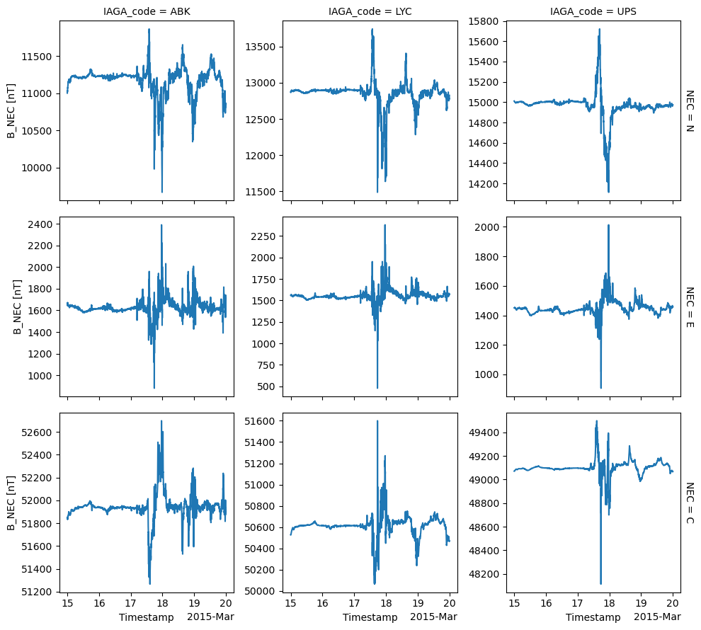
As well as access to Swarm data, VirES also provides access to ground observatory data from INTERMAGNET. We can fetch data from the minute resolution dataset (SW_OPER_AUX_OBSM2_), specifying desired observatories according to their 3-letter IAGA codes. These data have been rotated from the geodetic reference frame to the geocentric frame (NEC).
We’ll select three observatories in Sweden: Abisko (ABK), Lycksele (LYC) and Uppsala (UPS), which form a chain across about 10 degrees of latitude along a similar longitude.
def fetch_ground_obs(IAGA_codes, start_time, end_time):
    request = SwarmRequest()
    request.set_collection(
        *[f"SW_OPER_AUX_OBSM2_:{c}" for c in IAGA_codes], verbose=False
    )
    request.set_products(
        measurements=["B_NEC", "IAGA_code"],
    )
    data = request.get_between(
        start_time, end_time, asynchronous=False, show_progress=False
    )
    ds = data.as_xarray(reshape=True)
    return ds


ds_ground_obs = fetch_ground_obs(["ABK", "LYC", "UPS"], START_TIME, END_TIME)
ds_ground_obs
<xarray.Dataset>
Dimensions:    (Timestamp: 7200, IAGA_code: 3, NEC: 3)
Coordinates:
  * Timestamp  (Timestamp) datetime64[ns] 2015-03-15 ... 2015-03-19T23:59:00
    Latitude   (IAGA_code) float64 68.23 64.46 59.74
    Longitude  (IAGA_code) float64 18.82 18.75 17.35
    Radius     (IAGA_code) float64 6.36e+06 6.361e+06 6.362e+06
  * NEC        (NEC) <U1 'N' 'E' 'C'
  * IAGA_code  (IAGA_code) <U3 'ABK' 'LYC' 'UPS'
Data variables:
    B_NEC      (IAGA_code, Timestamp, NEC) float64 1.102e+04 ... 4.907e+04
Attributes:
    Sources:         ['SW_OPER_AUX_OBSM2__20150315T000000_20150315T235959_010...
    MagneticModels:  []
AppliedFilters: []By specifiying reshape=True when loading the xarray object, a multi-dimensional dataset is formed with a new IAGA_code axis. Here we show the three vector components from each observatory:
ds_ground_obs["B_NEC"].plot.line(
    x="Timestamp", row="NEC", col="IAGA_code", sharey=False
);

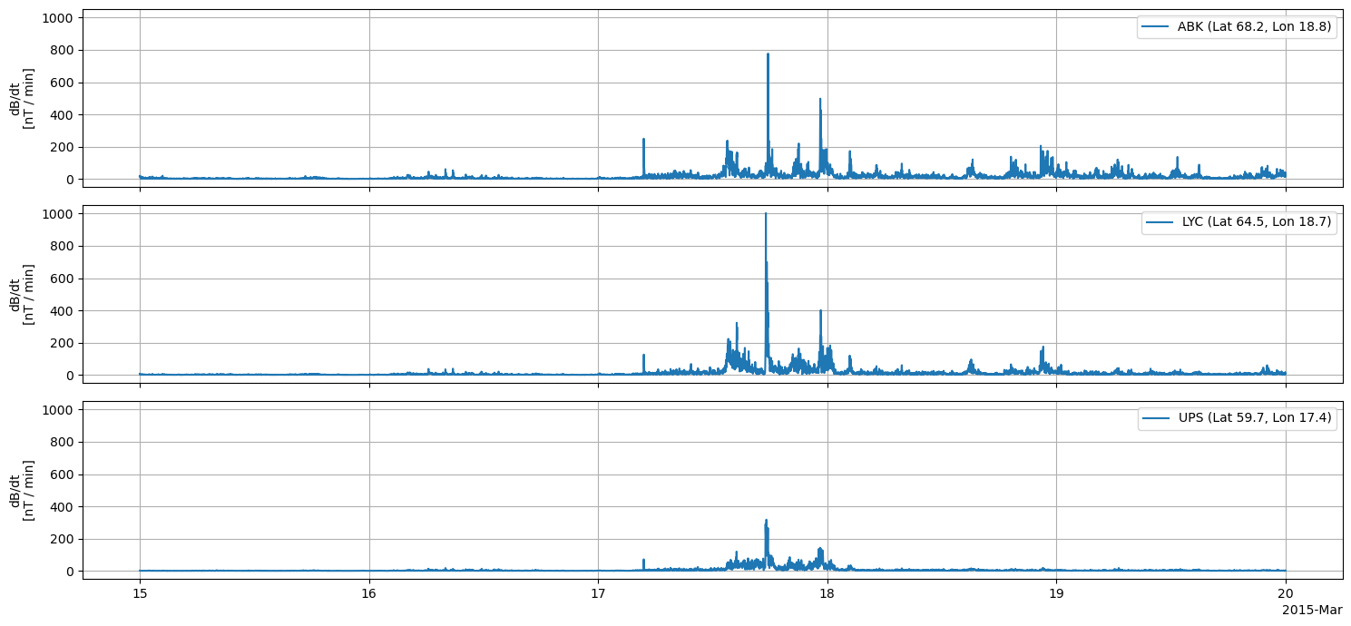
Let’s calculate \(|\frac{dB}{dt}|\) and plot that instead. This is a good indication of the GIC risk, as a more rapidly changing magnetic field will induce a larger electric field in the ground.
def plot_groundobs_dbdt(ds_ground_obs):
    ds_ground_obs = ds_ground_obs.assign(
        dBdt=(ds_ground_obs["B_NEC"].diff("Timestamp") ** 2)
        .sum(dim="NEC")
        .pipe(np.sqrt)
    )
    fig, axes = plt.subplots(nrows=3, figsize=(15, 7), sharey=True, sharex=True)
    for i, obs in enumerate(ds_ground_obs["IAGA_code"].values):
        _ds = ds_ground_obs.sel(IAGA_code=obs)
        lat = np.round(float(_ds["Latitude"]), 1)
        lon = np.round(float(_ds["Longitude"]), 1)
        label = f"{obs} (Lat {lat}, Lon {lon})"
        ds_ground_obs["dBdt"].sel(IAGA_code=obs).plot.line(
            x="Timestamp", ax=axes[i], label=label
        )
        axes[i].set_title("")
        axes[i].legend()
        axes[i].set_xlabel("")
        axes[i].set_ylabel("dB/dt\n[nT / min]")
        axes[i].grid()
        fig.tight_layout()
    return fig, axes


fig_grdbdt, axes_grdbdt = plot_groundobs_dbdt(ds_ground_obs)

