MAGxLR_1B (Magnetic field 1Hz)

Abstract: Access to the low rate (1Hz) magnetic data (level 1b product), together with geomagnetic model evaluations (level 2 products).

%load_ext watermark
%watermark -i -v -p viresclient,pandas,xarray,matplotlib

Python implementation: CPython
Python version       : 3.11.6
IPython version      : 8.18.0

viresclient: 0.15.0
pandas     : 2.1.3
xarray     : 2023.12.0
matplotlib : 3.8.2

from viresclient import SwarmRequest
import datetime as dt
import matplotlib.pyplot as plt

request = SwarmRequest()

Product information

This is one of the main products from Swarm - the 1Hz measurements of the magnetic field vector (B_NEC) and total intensity (F). These are derived from the Vector Field Magnetometer (VFM) and Absolute Scalar Magnetometer (ASM).

Documentation:

• Swarm Handbook: MAGx_LR_1B

• Product specification

Measurements are available through VirES as part of collections with names containing MAGx_LR, for each Swarm spacecraft:

request.available_collections("MAG", details=False)

{'MAG': ['SW_OPER_MAGA_LR_1B',
  'SW_OPER_MAGB_LR_1B',
  'SW_OPER_MAGC_LR_1B',
  'SW_FAST_MAGA_LR_1B',
  'SW_FAST_MAGB_LR_1B',
  'SW_FAST_MAGC_LR_1B']}

The measurements can be used together with geomagnetic model evaluations as shall be shown below.

Check what “MAG” data variables are available

request.available_measurements("MAG")

['F',
 'dF_Sun',
 'dF_AOCS',
 'dF_other',
 'F_error',
 'B_VFM',
 'B_NEC',
 'dB_Sun',
 'dB_AOCS',
 'dB_other',
 'B_error',
 'q_NEC_CRF',
 'Att_error',
 'Flags_F',
 'Flags_B',
 'Flags_q',
 'Flags_Platform',
 'ASM_Freq_Dev']

Check the names of available models

request.available_models(details=False)

['IGRF',
 'LCS-1',
 'MF7',
 'CHAOS-Core',
 'CHAOS-Static',
 'CHAOS-MMA-Primary',
 'CHAOS-MMA-Secondary',
 'CHAOS-MIO',
 'MCO_SHA_2C',
 'MCO_SHA_2D',
 'MLI_SHA_2C',
 'MLI_SHA_2D',
 'MLI_SHA_2E',
 'MMA_SHA_2C-Primary',
 'MMA_SHA_2C-Secondary',
 'MMA_SHA_2F-Primary',
 'MMA_SHA_2F-Secondary',
 'MIO_SHA_2C-Primary',
 'MIO_SHA_2C-Secondary',
 'MIO_SHA_2D-Primary',
 'MIO_SHA_2D-Secondary',
 'AMPS',
 'MCO_SHA_2X',
 'CHAOS',
 'CHAOS-MMA',
 'MMA_SHA_2C',
 'MMA_SHA_2F',
 'MIO_SHA_2C',
 'MIO_SHA_2D',
 'SwarmCI']

Fetch some MAG data and models

We can fetch the data and the model predictions (evaluated on demand) at the same time. We can also subsample the data - here we subsample it to 10-seconds by specifying the “PT10S” sampling_step.

request.set_collection("SW_OPER_MAGA_LR_1B")
request.set_products(
    measurements=["F", "B_NEC"],
    models=["CHAOS-Core", "MCO_SHA_2D"],
    sampling_step="PT10S",
)
data = request.get_between(
    # 2014-01-01 00:00:00
    start_time=dt.datetime(2014, 1, 1, 0),
    # 2014-01-01 01:00:00
    end_time=dt.datetime(2014, 1, 1, 1),
)

See a list of the source files

data.sources

['SW_OPER_MAGA_LR_1B_20140101T000000_20140101T235959_0701_MDR_MAG_LR',
 'SW_OPER_MCO_SHA_2D_20131126T000000_20180101T000000_0401',
 'SW_OPER_MCO_SHA_2X_19970101T000000_20260206T235959_0805']

Load as a pandas dataframe

Use expand=True to extract vectors (B_NEC…) as separate columns (…_N, …_E, …_C)

df = data.as_dataframe(expand=True)
df.head()

	Longitude	Radius	F_MCO_SHA_2D	F_CHAOS-Core	Spacecraft	F	Latitude	B_NEC_CHAOS-Core_N	B_NEC_CHAOS-Core_E	B_NEC_CHAOS-Core_C	B_NEC_N	B_NEC_E	B_NEC_C	B_NEC_MCO_SHA_2D_N	B_NEC_MCO_SHA_2D_E	B_NEC_MCO_SHA_2D_C
Timestamp
2014-01-01 00:00:00	-14.116674	6878309.23	22874.211386	22874.102418	A	22867.4800	-1.228938	20113.300310	-4127.295736	-10081.921542	20103.4954	-4125.6029	-10086.8732	20113.623790	-4127.463942	-10081.454557
2014-01-01 00:00:10	-14.131424	6878381.18	22820.941311	22820.824671	A	22814.4928	-1.862521	19824.823720	-4162.950034	-10508.865313	19815.0284	-4160.3663	-10514.3464	19825.161759	-4163.127529	-10508.410571
2014-01-01 00:00:20	-14.146155	6878452.06	22769.369047	22769.247190	A	22763.1833	-2.496090	19533.204562	-4197.343160	-10921.302465	19523.4054	-4194.6083	-10926.9383	19533.553823	-4197.529033	-10920.860399
2014-01-01 00:00:30	-14.160861	6878521.88	22719.238127	22719.113563	A	22713.2926	-3.129644	19238.986055	-4230.408364	-11319.151105	19229.1766	-4227.8647	-11324.7658	19239.343493	-4230.601798	-11318.721282
2014-01-01 00:00:40	-14.175534	6878590.62	22670.304568	22670.179741	A	22664.6401	-3.763184	18942.712049	-4262.080309	-11702.366477	18932.8056	-4260.1382	-11708.0771	18943.075066	-4262.280613	-11701.947711

… or as an xarray dataset:

ds = data.as_xarray()
ds

<xarray.Dataset>
Dimensions:           (Timestamp: 360, NEC: 3)
Coordinates:
  * Timestamp         (Timestamp) datetime64[ns] 2014-01-01 ... 2014-01-01T00...
  * NEC               (NEC) <U1 'N' 'E' 'C'
Data variables:
    Spacecraft        (Timestamp) object 'A' 'A' 'A' 'A' 'A' ... 'A' 'A' 'A' 'A'
    Longitude         (Timestamp) float64 -14.12 -14.13 -14.15 ... 153.6 153.6
    B_NEC             (Timestamp, NEC) float64 2.01e+04 -4.126e+03 ... 3.558e+04
    Radius            (Timestamp) float64 6.878e+06 6.878e+06 ... 6.868e+06
    B_NEC_MCO_SHA_2D  (Timestamp, NEC) float64 2.011e+04 ... 3.557e+04
    F_MCO_SHA_2D      (Timestamp) float64 2.287e+04 2.282e+04 ... 4.021e+04
    F_CHAOS-Core      (Timestamp) float64 2.287e+04 2.282e+04 ... 4.02e+04
    F                 (Timestamp) float64 2.287e+04 2.281e+04 ... 4.021e+04
    Latitude          (Timestamp) float64 -1.229 -1.863 -2.496 ... 48.14 48.77
    B_NEC_CHAOS-Core  (Timestamp, NEC) float64 2.011e+04 ... 3.557e+04
Attributes:
    Sources:         ['SW_OPER_MAGA_LR_1B_20140101T000000_20140101T235959_070...
    MagneticModels:  ["CHAOS-Core = 'CHAOS-Core'(max_degree=20,min_degree=1)"...
    AppliedFilters:  []

xarray.Dataset

• Dimensions:
  • Timestamp: 360
  • NEC: 3
• Coordinates: (2)
  • Timestamp
    (Timestamp)
    datetime64[ns]
    2014-01-01 ... 2014-01-01T00:59:50

    description :

    Time stamp

    array(['2014-01-01T00:00:00.000000000', '2014-01-01T00:00:10.000000000',
           '2014-01-01T00:00:20.000000000', ..., '2014-01-01T00:59:30.000000000',
           '2014-01-01T00:59:40.000000000', '2014-01-01T00:59:50.000000000'],
          dtype='datetime64[ns]')

  • NEC
    (NEC)
    <U1
    'N' 'E' 'C'

    units :

    description :

    NEC frame - North, East, Centre (down)

    array(['N', 'E', 'C'], dtype='<U1')

• Data variables: (10)
  • Spacecraft
    (Timestamp)
    object
    'A' 'A' 'A' 'A' ... 'A' 'A' 'A' 'A'

    units :

    -

    description :

    Spacecraft identifier (values: 'A', 'B', 'C' or '-' if not available).

    array(['A', 'A', 'A', 'A', 'A', 'A', 'A', 'A', 'A', 'A', 'A', 'A', 'A',
           'A', 'A', 'A', 'A', 'A', 'A', 'A', 'A', 'A', 'A', 'A', 'A', 'A',
           'A', 'A', 'A', 'A', 'A', 'A', 'A', 'A', 'A', 'A', 'A', 'A', 'A',
           'A', 'A', 'A', 'A', 'A', 'A', 'A', 'A', 'A', 'A', 'A', 'A', 'A',
           'A', 'A', 'A', 'A', 'A', 'A', 'A', 'A', 'A', 'A', 'A', 'A', 'A',
           'A', 'A', 'A', 'A', 'A', 'A', 'A', 'A', 'A', 'A', 'A', 'A', 'A',
           'A', 'A', 'A', 'A', 'A', 'A', 'A', 'A', 'A', 'A', 'A', 'A', 'A',
           'A', 'A', 'A', 'A', 'A', 'A', 'A', 'A', 'A', 'A', 'A', 'A', 'A',
           'A', 'A', 'A', 'A', 'A', 'A', 'A', 'A', 'A', 'A', 'A', 'A', 'A',
           'A', 'A', 'A', 'A', 'A', 'A', 'A', 'A', 'A', 'A', 'A', 'A', 'A',
           'A', 'A', 'A', 'A', 'A', 'A', 'A', 'A', 'A', 'A', 'A', 'A', 'A',
           'A', 'A', 'A', 'A', 'A', 'A', 'A', 'A', 'A', 'A', 'A', 'A', 'A',
           'A', 'A', 'A', 'A', 'A', 'A', 'A', 'A', 'A', 'A', 'A', 'A', 'A',
           'A', 'A', 'A', 'A', 'A', 'A', 'A', 'A', 'A', 'A', 'A', 'A', 'A',
           'A', 'A', 'A', 'A', 'A', 'A', 'A', 'A', 'A', 'A', 'A', 'A', 'A',
           'A', 'A', 'A', 'A', 'A', 'A', 'A', 'A', 'A', 'A', 'A', 'A', 'A',
           'A', 'A', 'A', 'A', 'A', 'A', 'A', 'A', 'A', 'A', 'A', 'A', 'A',
           'A', 'A', 'A', 'A', 'A', 'A', 'A', 'A', 'A', 'A', 'A', 'A', 'A',
           'A', 'A', 'A', 'A', 'A', 'A', 'A', 'A', 'A', 'A', 'A', 'A', 'A',
           'A', 'A', 'A', 'A', 'A', 'A', 'A', 'A', 'A', 'A', 'A', 'A', 'A',
           'A', 'A', 'A', 'A', 'A', 'A', 'A', 'A', 'A', 'A', 'A', 'A', 'A',
           'A', 'A', 'A', 'A', 'A', 'A', 'A', 'A', 'A', 'A', 'A', 'A', 'A',
           'A', 'A', 'A', 'A', 'A', 'A', 'A', 'A', 'A', 'A', 'A', 'A', 'A',
           'A', 'A', 'A', 'A', 'A', 'A', 'A', 'A', 'A', 'A', 'A', 'A', 'A',
           'A', 'A', 'A', 'A', 'A', 'A', 'A', 'A', 'A', 'A', 'A', 'A', 'A',
           'A', 'A', 'A', 'A', 'A', 'A', 'A', 'A', 'A', 'A', 'A', 'A', 'A',
           'A', 'A', 'A', 'A', 'A', 'A', 'A', 'A', 'A', 'A', 'A', 'A', 'A',
           'A', 'A', 'A', 'A', 'A', 'A', 'A', 'A', 'A'], dtype=object)

  • Longitude
    (Timestamp)
    float64
    -14.12 -14.13 ... 153.6 153.6

    units :

    deg

    description :

    Position in ITRF - Longitude

    array([-14.1166743, -14.1314243, -14.1461554, -14.1608609, -14.1755342,
           -14.1901685, -14.2047571, -14.2192932, -14.2337699, -14.2481804,
           -14.2625177, -14.2767748, -14.2909444, -14.3050195, -14.3189927,
           -14.3328566, -14.3466037, -14.3602264, -14.3737168, -14.3870671,
           -14.4002693, -14.4133151, -14.4261961, -14.4389038, -14.4514295,
           -14.4637642, -14.4758988, -14.4878238, -14.4995298, -14.5110068,
           -14.5222447, -14.5332332, -14.5439615, -14.5544187, -14.5645933,
           -14.5744739, -14.5840483, -14.5933041, -14.6022285, -14.6108083,
           -14.6190299, -14.6268789, -14.6343409, -14.6414006, -14.6480422,
           -14.6542495, -14.6600055, -14.6652927, -14.6700926, -14.6743864,
           -14.6781542, -14.6813754, -14.6840285, -14.6860912, -14.6875401,
           -14.6883507, -14.6884977, -14.6879543, -14.6866927, -14.6846837,
           -14.6818967, -14.6782997, -14.673859 , -14.6685394, -14.6623038,
           -14.6551131, -14.6469263, -14.6377003, -14.6273894, -14.6159457,
           -14.6033184, -14.589454 , -14.5742958, -14.557784 , -14.539855 ,
           -14.5204415, -14.4994721, -14.476871 , -14.4525575, -14.4264457,
           -14.3984442, -14.3684554, -14.3363752, -14.3020922, -14.2654873,
           -14.2264328, -14.1847917, -14.1404169, -14.0931501, -14.0428207,
           -13.989245 , -13.9322242, -13.8715433, -13.8069696, -13.73825  ,
           -13.6651097, -13.5872493, -13.5043418, -13.41603  , -13.3219222,
    ...
           154.3456616, 154.3325292, 154.3192466, 154.3058218, 154.2922629,
           154.2785777, 154.2647737, 154.2508587, 154.23684  , 154.222725 ,
           154.2085209, 154.1942349, 154.1798741, 154.1654455, 154.1509559,
           154.1364123, 154.1218215, 154.1071902, 154.0925253, 154.0778333,
           154.063121 , 154.048395 , 154.033662 , 154.0189287, 154.0042015,
           153.9894873, 153.9747926, 153.9601241, 153.9454886, 153.9308927,
           153.9163432, 153.901847 , 153.8874109, 153.8730419, 153.8587469,
           153.8445331, 153.8304075, 153.8163774, 153.8024502, 153.7886334,
           153.7749344, 153.761361 , 153.7479209, 153.7346221, 153.7214728,
           153.7084812, 153.6956557, 153.6830049, 153.6705376, 153.6582628,
           153.6461898, 153.634328 , 153.622687 , 153.6112768, 153.6001075,
           153.5891898, 153.5785343, 153.5681521, 153.5580546, 153.5482537,
           153.5387614, 153.5295904, 153.5207534, 153.5122638, 153.5041356,
           153.496383 , 153.4890208, 153.4820643, 153.4755295, 153.4694328,
           153.4637914, 153.4586231, 153.4539463, 153.4497804, 153.4461453,
           153.443062 , 153.4405521, 153.4386383, 153.4373443, 153.4366949,
           153.4367157, 153.4374339, 153.4388777, 153.4410767, 153.4440618,
           153.4478657, 153.4525224, 153.4580678, 153.4645395, 153.4719771,
           153.4804224, 153.4899192, 153.5005138, 153.5122551, 153.5251946,
           153.5393868, 153.5548894, 153.5717634, 153.5900733, 153.6098879])

  • B_NEC
    (Timestamp, NEC)
    float64
    2.01e+04 -4.126e+03 ... 3.558e+04

    units :

    nT

    description :

    Magnetic field vector, NEC frame

    array([[ 20103.4954,  -4125.6029, -10086.8732],
           [ 19815.0284,  -4160.3663, -10514.3464],
           [ 19523.4054,  -4194.6083, -10926.9383],
           ...,
           [ 19122.1554,  -1771.8435,  34719.1592],
           [ 18879.7226,  -1789.2399,  35154.9347],
           [ 18635.0677,  -1804.4639,  35583.8968]])

  • Radius
    (Timestamp)
    float64
    6.878e+06 6.878e+06 ... 6.868e+06

    units :

    m

    description :

    Position in ITRF - Radius

    array([6878309.23, 6878381.18, 6878452.06, 6878521.88, 6878590.62,
           6878658.28, 6878724.85, 6878790.33, 6878854.71, 6878917.98,
           6878980.14, 6879041.19, 6879101.13, 6879159.94, 6879217.64,
           6879274.21, 6879329.65, 6879383.96, 6879437.15, 6879489.2 ,
           6879540.13, 6879589.92, 6879638.58, 6879686.12, 6879732.52,
           6879777.8 , 6879821.96, 6879864.99, 6879906.9 , 6879947.69,
           6879987.37, 6880025.93, 6880063.39, 6880099.75, 6880135.01,
           6880169.17, 6880202.25, 6880234.24, 6880265.16, 6880295.  ,
           6880323.78, 6880351.5 , 6880378.17, 6880403.8 , 6880428.39,
           6880451.95, 6880474.49, 6880496.01, 6880516.54, 6880536.07,
           6880554.61, 6880572.18, 6880588.78, 6880604.42, 6880619.12,
           6880632.88, 6880645.71, 6880657.63, 6880668.64, 6880678.76,
           6880687.99, 6880696.36, 6880703.86, 6880710.51, 6880716.33,
           6880721.32, 6880725.5 , 6880728.88, 6880731.47, 6880733.28,
           6880734.34, 6880734.64, 6880734.21, 6880733.05, 6880731.18,
           6880728.61, 6880725.36, 6880721.44, 6880716.86, 6880711.63,
           6880705.78, 6880699.3 , 6880692.23, 6880684.56, 6880676.31,
           6880667.5 , 6880658.14, 6880648.24, 6880637.81, 6880626.88,
           6880615.45, 6880603.54, 6880591.15, 6880578.3 , 6880565.02,
           6880551.29, 6880537.16, 6880522.61, 6880507.67, 6880492.36,
    ...
           6875648.21, 6875587.21, 6875525.54, 6875463.21, 6875400.22,
           6875336.57, 6875272.26, 6875207.3 , 6875141.68, 6875075.42,
           6875008.52, 6874940.98, 6874872.8 , 6874804.  , 6874734.58,
           6874664.55, 6874593.9 , 6874522.66, 6874450.83, 6874378.4 ,
           6874305.41, 6874231.84, 6874157.71, 6874083.03, 6874007.82,
           6873932.07, 6873855.8 , 6873779.02, 6873701.74, 6873623.97,
           6873545.73, 6873467.02, 6873387.86, 6873308.26, 6873228.24,
           6873147.8 , 6873066.96, 6872985.74, 6872904.15, 6872822.2 ,
           6872739.91, 6872657.3 , 6872574.37, 6872491.16, 6872407.66,
           6872323.9 , 6872239.9 , 6872155.67, 6872071.23, 6871986.6 ,
           6871901.79, 6871816.82, 6871731.71, 6871646.48, 6871561.14,
           6871475.72, 6871390.23, 6871304.7 , 6871219.15, 6871133.59,
           6871048.04, 6870962.54, 6870877.08, 6870791.71, 6870706.43,
           6870621.28, 6870536.27, 6870451.42, 6870366.75, 6870282.3 ,
           6870198.07, 6870114.09, 6870030.39, 6869946.98, 6869863.89,
           6869781.14, 6869698.75, 6869616.75, 6869535.15, 6869453.98,
           6869373.26, 6869293.01, 6869213.27, 6869134.03, 6869055.34,
           6868977.21, 6868899.67, 6868822.73, 6868746.41, 6868670.75,
           6868595.76, 6868521.47, 6868447.89, 6868375.05, 6868302.96,
           6868231.66, 6868161.16, 6868091.48, 6868022.65, 6867954.68])

  • B_NEC_MCO_SHA_2D
    (Timestamp, NEC)
    float64
    2.011e+04 -4.127e+03 ... 3.557e+04

    units :

    nT

    description :

    Magnetic field vector, NEC frame, calculated by the MCO_SHA_2D spherical harmonic model

    array([[ 20113.62378973,  -4127.46394188, -10081.45455737],
           [ 19825.16175918,  -4163.12752932, -10508.41057114],
           [ 19533.55382342,  -4197.52903345, -10920.86039864],
           ...,
           [ 19129.93319584,  -1775.95410044,  34711.24757684],
           [ 18889.68968635,  -1793.32968584,  35145.82174384],
           [ 18645.41210832,  -1808.14125488,  35574.78759174]])

  • F_MCO_SHA_2D
    (Timestamp)
    float64
    2.287e+04 2.282e+04 ... 4.021e+04

    units :

    nT

    description :

    Magnetic field intensity, calculated by the MCO_SHA_2D spherical harmonic model

    array([22874.21138616, 22820.94131132, 22769.36904716, 22719.23812689,
           22670.30456813, 22622.33780792, 22575.12219399, 22528.45785223,
           22482.16170451, 22436.06798846, 22390.02860622, 22343.91347663,
           22297.61065434, 22251.02639378, 22204.08431774, 22156.72588855,
           22108.9092914 , 22060.60902499, 22011.81515049, 21962.53291883,
           21912.7812344 , 21862.59267082, 21812.01183649, 21761.09481799,
           21709.90856487, 21658.52935921, 21607.04251047, 21555.5415094 ,
           21504.1268485 , 21452.90569329, 21401.99095358, 21351.50091329,
           21301.55828264, 21252.29007445, 21203.827063  , 21156.30328653,
           21109.85571902, 21064.62434957, 21020.75151474, 20978.38227606,
           20937.66387404, 20898.74611749, 20861.78114204, 20826.92361666,
           20794.33090157, 20764.16301399, 20736.58291589, 20711.75672146,
           20689.85359818, 20671.04643809, 20655.51157698, 20643.42899529,
           20634.98262621, 20630.36018213, 20629.75315604, 20633.35696346,
           20641.37057624, 20653.99633765, 20671.43985026, 20693.90933254,
           20721.61542764, 20754.77031082, 20793.58752921, 20838.28078812,
           20889.06339288, 20946.14745762, 21009.74272677, 21080.05574657,
           21157.28874098, 21241.63851139, 21333.2951812 , 21432.44141394,
           21539.25067184, 21653.88661456, 21776.50147754, 21907.23524988,
           22046.21440529, 22193.55091641, 22349.34139861, 22513.66597902,
    ...
           29753.73149158, 29567.29858251, 29389.91738895, 29221.81070888,
           29063.18672034, 28914.23907109, 28775.14579608, 28646.06946135,
           28527.1568092 , 28418.53851618, 28320.32879594, 28232.62565262,
           28155.51015437, 28089.04674398, 28033.28286664, 27988.24922   ,
           27953.9593535 , 27930.40982301, 27917.58043007, 27915.43419568,
           27923.91743863, 27942.96007831, 27972.47621988, 28012.36375455,
           28062.50589802, 28122.77063892, 28193.01188183, 28273.07017952,
           28362.77312409, 28461.93639944, 28570.36464514, 28687.85223957,
           28814.18435767, 28949.13790944, 29092.48279928, 29243.9824857 ,
           29403.39552589, 29570.4760846 , 29744.97520543, 29926.64166522,
           30115.22265463, 30310.46417701, 30512.11274767, 30719.91435924,
           30933.61629806, 31152.96636296, 31377.71381857, 31607.60912575,
           31842.40381692, 32081.850296  , 32325.70244284, 32573.71430537,
           32825.64048263, 33081.23589554, 33340.25506546, 33602.45237909,
           33867.58157525, 34135.39554529, 34405.64657939, 34678.08596949,
           34952.46434901, 35228.53161871, 35506.03702845, 35784.73038678,
           36064.36077272, 36344.67833413, 36625.43397114, 36906.38002846,
           37187.27052549, 37467.86123988, 37747.91074114, 38027.18003385,
           38305.43319013, 38582.43709407, 38857.96187529, 39131.78027805,
           39403.66844511, 39673.40501375, 39940.77107241, 40205.55035918])

  • F_CHAOS-Core
    (Timestamp)
    float64
    2.287e+04 2.282e+04 ... 4.02e+04

    units :

    nT

    description :

    Magnetic field intensity, calculated by the CHAOS-Core spherical harmonic model

    array([22874.10241801, 22820.82467125, 22769.2471898 , 22719.11356342,
           22670.17974121, 22622.21497026, 22575.00329535, 22528.34443914,
           22482.05483676, 22435.96817563, 22389.93576674, 22343.82692123,
           22297.52909433, 22250.94797408, 22204.00667316, 22156.6462211 ,
           22108.82446538, 22060.51567593, 22011.70980345, 21962.41211099,
           21912.64163694, 21862.431205  , 21811.82577901, 21760.88189156,
           21709.66701014, 21658.25798551, 21606.7407235 , 21555.20931526,
           21503.76483444, 21452.51498672, 21401.57316183, 21351.05804753,
           21301.09267   , 21251.80426297, 21203.32372424, 21155.78512057,
           21109.3253666 , 21064.08431534, 21020.20410505, 20977.82955371,
           20937.10763158, 20898.18786922, 20861.22213407, 20826.36485307,
           20793.77318378, 20763.60698962, 20736.02913282, 20711.20568231,
           20689.30581043, 20670.50245528, 20654.97202673, 20642.89459093,
           20634.45415953, 20629.83849605, 20629.23909735, 20632.85131701,
           20640.87398337, 20653.50920292, 20670.96224151, 20693.44088022,
           20721.15522983, 20754.31685049, 20793.13861017, 20837.83349554,
           20888.6140831 , 20945.69178113, 21009.27568628, 21079.57179058,
           21156.78189142, 21241.10252189, 21332.72372092, 21431.82827022,
           21538.58996366, 21653.1730077 , 21775.73039212, 21906.40305044,
           22045.31856452, 22192.5901441 , 22348.31572892, 22512.57681098,
    ...
           29753.09615788, 29566.6884719 , 29389.33287779, 29221.25211478,
           29062.65432088, 28913.73311884, 28774.66652896, 28645.6171074 ,
           28526.73158541, 28418.14062131, 28319.95839778, 28232.28287032,
           28155.19503712, 28088.75924717, 28033.02282745, 27988.01633392,
           27953.75315378, 27930.22966471, 27917.42548051, 27915.30343263,
           27923.80965736, 27942.87390827, 27972.4101512 , 28012.31617406,
           28062.47513405, 28122.75501342, 28193.00976796, 28273.08006228,
           28362.79366122, 28461.96647951, 28570.40343957, 28687.89924524,
           28814.23942706, 28949.20126533, 29092.55503174, 29244.06452947,
           29403.48861735, 29570.58169807, 29745.09496977, 29926.77726263,
           30115.3757046 , 30310.63610921, 30512.30466883, 30720.12691916,
           30933.84956112, 31153.21969119, 31377.98577281, 31607.89739068,
           31842.70515565, 32082.16053851, 32326.01651186, 32574.02628137,
           32825.94370837, 33081.5231186 , 33340.51861547, 33602.68437448,
           33867.77415271, 34135.54110347, 34405.73802738, 34678.11696933,
           34952.4295415 , 35228.42682136, 35505.85939507, 35784.47851935,
           36064.03477728, 36344.27981484, 36624.96595864, 36905.84684151,
           37186.67756768, 37467.21473611, 37747.21742166, 38026.44677629,
           38304.66663246, 38581.64323353, 38857.14566988, 39130.94526799,
           39402.81641196, 39672.53569421, 39939.88194264, 40204.63650322])

  • F
    (Timestamp)
    float64
    2.287e+04 2.281e+04 ... 4.021e+04

    units :

    nT

    description :

    Magnetic field intensity

    array([22867.48  , 22814.4928, 22763.1833, 22713.2926, 22664.6401,
           22616.981 , 22570.0902, 22523.7412, 22477.8273, 22431.8837,
           22386.1082, 22340.259 , 22294.2376, 22247.9259, 22201.2616,
           22154.1974, 22106.6763, 22058.6843, 22010.1957, 21961.2106,
           21911.7308, 21861.8112, 21811.4803, 21760.8121, 21709.8413,
           21658.6641, 21607.3722, 21556.0581, 21504.8344, 21453.7973,
           21403.0866, 21352.8112, 21303.0841, 21254.0392, 21205.8074,
           21158.5097, 21112.2957, 21067.2896, 21023.6259, 20981.4687,
           20940.9486, 20902.2263, 20865.4504, 20830.7853, 20798.3563,
           20768.351 , 20740.9447, 20716.2807, 20694.5331, 20675.8817,
           20660.5088, 20648.5955, 20640.3487, 20635.9422, 20635.553 ,
           20639.3701, 20647.5942, 20660.4089, 20678.0156, 20700.6294,
           20728.4632, 20761.7408, 20800.6806, 20845.5159, 20896.4612,
           20953.7202, 21017.5213, 21088.0509, 21165.5046, 21250.0801,
           21341.9487, 21441.3026, 21548.2969, 21663.0908, 21785.8488,
           21916.694 , 22055.7687, 22203.1876, 22359.0756, 22523.4809,
           22696.4748, 22878.1026, 23068.3912, 23267.2875, 23474.8191,
           23690.9183, 23915.5855, 24148.7173, 24390.2364, 24640.0689,
           24898.0557, 25164.0728, 25438.0294, 25719.8477, 26009.3117,
           26306.3028, 26610.5514, 26921.883 , 27240.0086, 27564.4736,
    ...
           34918.218 , 34614.28  , 34313.0986, 34014.9786, 33720.2617,
           33429.2172, 33142.1549, 32859.3547, 32581.1846, 32308.0043,
           32040.1895, 31778.161 , 31522.4024, 31273.3331, 31031.3344,
           30796.7383, 30569.7476, 30350.5639, 30139.3461, 29936.3048,
           29741.6012, 29555.5005, 29378.1374, 29209.6813, 29050.3407,
           28900.3185, 28759.7337, 28628.8479, 28507.9192, 28397.2353,
           28297.0672, 28207.7394, 28129.598 , 28062.9408, 28007.9166,
           27964.5242, 27932.6141, 27911.8936, 27902.0391, 27902.7298,
           27913.7127, 27934.81  , 27965.8664, 28006.8241, 28057.6229,
           28118.2251, 28188.5707, 28268.5615, 28358.1156, 28457.1152,
           28565.386 , 28682.7183, 28808.8774, 28943.6009, 29086.7143,
           29238.0311, 29397.3284, 29564.3195, 29738.7628, 29920.4256,
           30109.0907, 30304.4719, 30506.3303, 30714.4171, 30928.4058,
           31148.031 , 31372.9719, 31603.0024, 31837.8207, 32077.2016,
           32320.914 , 32568.7454, 32820.4338, 33075.8282, 33334.7721,
           33597.0544, 33862.3692, 34130.4565, 34401.0478, 34673.8957,
           34948.6925, 35225.2049, 35503.182 , 35782.3348, 36062.4514,
           36343.3008, 36624.6366, 36906.1407, 37187.551 , 37468.5674,
           37748.9645, 38028.4886, 38306.9624, 38584.1935, 38860.0058,
           39134.1305, 39406.3438, 39676.3845, 39943.8931, 40208.6267])

  • Latitude
    (Timestamp)
    float64
    -1.229 -1.863 ... 48.14 48.77

    units :

    deg

    description :

    Position in ITRF - Latitude

    array([ -1.2289378,  -1.8625209,  -2.4960899,  -3.1296444,  -3.7631844,
            -4.3967096,  -5.03022  ,  -5.6637153,  -6.2971954,  -6.9306601,
            -7.5641093,  -8.1975429,  -8.8309607,  -9.4643624, -10.097748 ,
           -10.7311174, -11.3644703, -11.9978066, -12.6311262, -13.2644288,
           -13.8977144, -14.5309828, -15.1642339, -15.7974674, -16.4306832,
           -17.0638811, -17.6970611, -18.3302228, -18.9633662, -19.5964911,
           -20.2295972, -20.8626845, -21.4957527, -22.1288017, -22.7618311,
           -23.394841 , -24.027831 , -24.6608009, -25.2937505, -25.9266797,
           -26.5595881, -27.1924756, -27.8253419, -28.4581867, -29.0910097,
           -29.7238108, -30.3565896, -30.9893458, -31.6220792, -32.2547893,
           -32.8874759, -33.5201386, -34.1527771, -34.7853909, -35.4179797,
           -36.0505431, -36.6830805, -37.3155916, -37.9480759, -38.5805328,
           -39.2129618, -39.8453623, -40.4777338, -41.1100755, -41.7423869,
           -42.3746672, -43.0069157, -43.6391316, -44.271314 , -44.903462 ,
           -45.5355747, -46.1676512, -46.7996902, -47.4316908, -48.0636516,
           -48.6955714, -49.3274489, -49.9592824, -50.5910706, -51.2228116,
           -51.8545038, -52.4861451, -53.1177335, -53.7492668, -54.3807426,
           -55.0121584, -55.6435114, -56.2747985, -56.9060167, -57.5371623,
           -58.1682317, -58.7992208, -59.4301252, -60.06094  , -60.69166  ,
           -61.3222795, -61.9527922, -62.5831914, -63.2134696, -63.8436184,
    ...
           -14.0397279, -13.4057211, -12.7716953, -12.1376508, -11.5035876,
           -10.8695063, -10.2354069,  -9.6012897,  -8.967155 ,  -8.333003 ,
            -7.6988341,  -7.0646483,  -6.4304461,  -5.7962276,  -5.161993 ,
            -4.5277427,  -3.8934769,  -3.2591959,  -2.6248998,  -1.990589 ,
            -1.3562637,  -0.7219241,  -0.0875706,   0.5467966,   1.1811773,
             1.8155712,   2.449978 ,   3.0843975,   3.7188294,   4.3532734,
             4.9877293,   5.6221967,   6.2566755,   6.8911653,   7.5256657,
             8.1601767,   8.7946978,   9.4292288,  10.0637693,  10.6983191,
            11.3328779,  11.9674454,  12.6020212,  13.2366051,  13.8711967,
            14.5057958,  15.1404019,  15.7750149,  16.4096342,  17.0442597,
            17.6788909,  18.3135275,  18.9481692,  19.5828155,  20.2174661,
            20.8521207,  21.4867788,  22.1214401,  22.7561042,  23.3907706,
            24.025439 ,  24.6601089,  25.2947799,  25.9294516,  26.5641235,
            27.1987952,  27.8334661,  28.4681359,  29.102804 ,  29.7374699,
            30.3721332,  31.0067932,  31.6414495,  32.2761015,  32.9107485,
            33.5453901,  34.1800256,  34.8146544,  35.4492757,  36.083889 ,
            36.7184936,  37.3530887,  37.9876736,  38.6222475,  39.2568096,
            39.891359 ,  40.525895 ,  41.1604165,  41.7949226,  42.4294124,
            43.0638848,  43.6983388,  44.3327731,  44.9671867,  45.6015782,
            46.2359464,  46.87029  ,  47.5046074,  48.1388971,  48.7731577])

  • B_NEC_CHAOS-Core
    (Timestamp, NEC)
    float64
    2.011e+04 -4.127e+03 ... 3.557e+04

    units :

    nT

    description :

    Magnetic field vector, NEC frame, calculated by the CHAOS-Core spherical harmonic model

    array([[ 20113.30031006,  -4127.29573596, -10081.92154177],
           [ 19824.82372012,  -4162.95003387, -10508.86531257],
           [ 19533.20456173,  -4197.34316005, -10921.30246519],
           ...,
           [ 19127.81397833,  -1776.15858279,  34711.41140184],
           [ 18887.52841803,  -1793.51471715,  35145.96342128],
           [ 18643.19829511,  -1808.31185008,  35574.90635178]])

• Indexes: (2)
  • Timestamp
    PandasIndex

    PandasIndex(DatetimeIndex(['2014-01-01 00:00:00', '2014-01-01 00:00:10',
                   '2014-01-01 00:00:20', '2014-01-01 00:00:30',
                   '2014-01-01 00:00:40', '2014-01-01 00:00:50',
                   '2014-01-01 00:01:00', '2014-01-01 00:01:10',
                   '2014-01-01 00:01:20', '2014-01-01 00:01:30',
                   ...
                   '2014-01-01 00:58:20', '2014-01-01 00:58:30',
                   '2014-01-01 00:58:40', '2014-01-01 00:58:50',
                   '2014-01-01 00:59:00', '2014-01-01 00:59:10',
                   '2014-01-01 00:59:20', '2014-01-01 00:59:30',
                   '2014-01-01 00:59:40', '2014-01-01 00:59:50'],
                  dtype='datetime64[ns]', name='Timestamp', length=360, freq=None))

  • NEC
    PandasIndex

    PandasIndex(Index(['N', 'E', 'C'], dtype='object', name='NEC'))

• Attributes: (3)

  Sources :

  ['SW_OPER_MAGA_LR_1B_20140101T000000_20140101T235959_0701_MDR_MAG_LR', 'SW_OPER_MCO_SHA_2D_20131126T000000_20180101T000000_0401', 'SW_OPER_MCO_SHA_2X_19970101T000000_20260206T235959_0805']

  MagneticModels :

  ["CHAOS-Core = 'CHAOS-Core'(max_degree=20,min_degree=1)", 'MCO_SHA_2D = MCO_SHA_2D(max_degree=20,min_degree=1)']

  AppliedFilters :

  []

Fetch the residuals directly

Adding residuals=True to .set_products() will instead directly evaluate and return all data-model residuals

request = SwarmRequest()
request.set_collection("SW_OPER_MAGA_LR_1B")
request.set_products(
    measurements=["F", "B_NEC"],
    models=["CHAOS-Core", "MCO_SHA_2D"],
    residuals=True,
    sampling_step="PT10S",
)
data = request.get_between(
    start_time=dt.datetime(2014, 1, 1, 0), end_time=dt.datetime(2014, 1, 1, 1)
)
df = data.as_dataframe(expand=True)
df.head()

	Longitude	Radius	Spacecraft	Latitude	F_res_CHAOS-Core	F_res_MCO_SHA_2D	B_NEC_res_CHAOS-Core_N	B_NEC_res_CHAOS-Core_E	B_NEC_res_CHAOS-Core_C	B_NEC_res_MCO_SHA_2D_N	B_NEC_res_MCO_SHA_2D_E	B_NEC_res_MCO_SHA_2D_C
Timestamp
2014-01-01 00:00:00	-14.116674	6878309.23	A	-1.228938	-6.622418	-6.731386	-9.804910	1.692836	-4.951658	-10.128390	1.861042	-5.418643
2014-01-01 00:00:10	-14.131424	6878381.18	A	-1.862521	-6.331871	-6.448511	-9.795320	2.583734	-5.481087	-10.133359	2.761229	-5.935829
2014-01-01 00:00:20	-14.146155	6878452.06	A	-2.496090	-6.063890	-6.185747	-9.799162	2.734860	-5.635835	-10.148423	2.920733	-6.077901
2014-01-01 00:00:30	-14.160861	6878521.88	A	-3.129644	-5.820963	-5.945527	-9.809455	2.543664	-5.614695	-10.166893	2.737098	-6.044518
2014-01-01 00:00:40	-14.175534	6878590.62	A	-3.763184	-5.539641	-5.664468	-9.906449	1.942109	-5.710623	-10.269466	2.142413	-6.129389

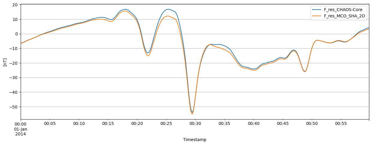
Plot the scalar residuals

… using the pandas method:

ax = df.plot(y=["F_res_CHAOS-Core", "F_res_MCO_SHA_2D"], figsize=(15, 5), grid=True)
ax.set_xlabel("Timestamp")
ax.set_ylabel("[nT]");

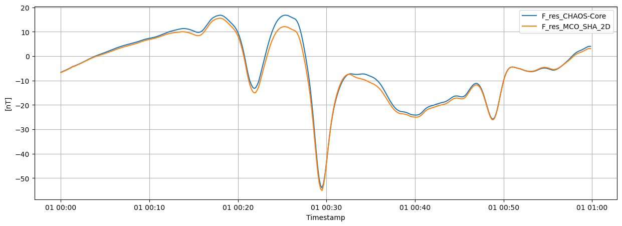
… using matplotlib interface

NB: we are doing plt.plot(x, y) with x as df.index (the time-based index of df), and y as df[".."]

plt.figure(figsize=(15, 5))
plt.plot(df.index, df["F_res_CHAOS-Core"], label="F_res_CHAOS-Core")
plt.plot(df.index, df["F_res_MCO_SHA_2D"], label="F_res_MCO_SHA_2D")
plt.xlabel("Timestamp")
plt.ylabel("[nT]")
plt.grid()
plt.legend();

… using matplotlib interface (Object Oriented style)

This is the recommended route for making more complicated figures

fig, ax = plt.subplots(figsize=(15, 5))
ax.plot(df.index, df["F_res_CHAOS-Core"], label="F_res_CHAOS-Core")
ax.plot(df.index, df["F_res_MCO_SHA_2D"], label="F_res_MCO_SHA_2D")
ax.set_xlabel("Timestamp")
ax.set_ylabel("[nT]")
ax.grid()
ax.legend();

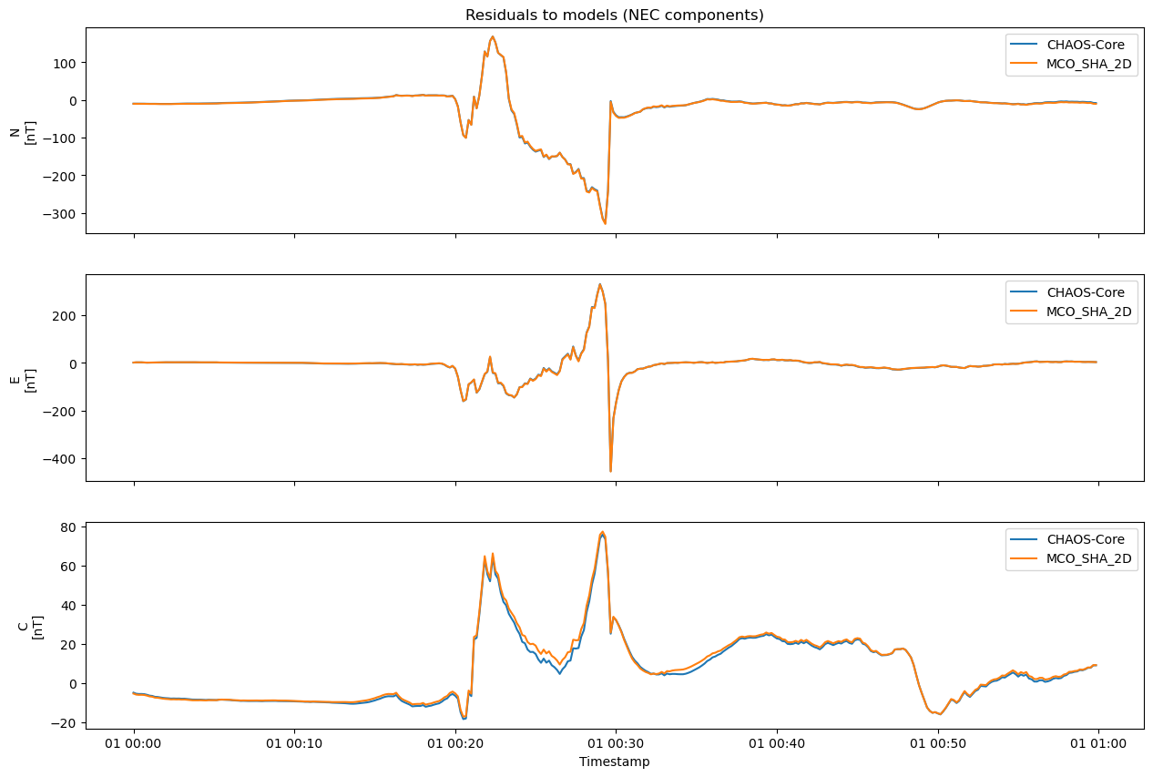
Plot the vector components

fig, axes = plt.subplots(nrows=3, ncols=1, figsize=(15, 10), sharex=True)
for component, ax in zip("NEC", axes):
    for model_name in ("CHAOS-Core", "MCO_SHA_2D"):
        ax.plot(df.index, df[f"B_NEC_res_{model_name}_{component}"], label=model_name)
    ax.set_ylabel(f"{component}\n[nT]")
    ax.legend()
axes[0].set_title("Residuals to models (NEC components)")
axes[2].set_xlabel("Timestamp");

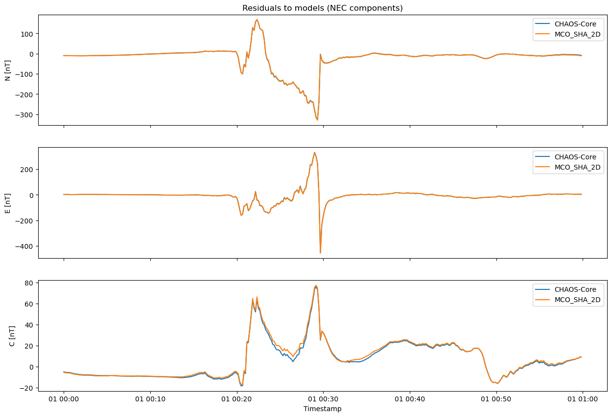
Similar plotting, using the data via xarray instead

xarray provides a more sophisticated data structure that is more suitable for the complex vector data we are accessing, together with nice stuff like unit and other metadata support. Unfortunately due to the extra complexity, this can make it difficult to use right away.

ds = data.as_xarray()
ds

<xarray.Dataset>
Dimensions:               (Timestamp: 360, NEC: 3)
Coordinates:
  * Timestamp             (Timestamp) datetime64[ns] 2014-01-01 ... 2014-01-0...
  * NEC                   (NEC) <U1 'N' 'E' 'C'
Data variables:
    Spacecraft            (Timestamp) object 'A' 'A' 'A' 'A' ... 'A' 'A' 'A' 'A'
    B_NEC_res_CHAOS-Core  (Timestamp, NEC) float64 -9.805 1.693 ... 3.848 8.99
    Longitude             (Timestamp) float64 -14.12 -14.13 ... 153.6 153.6
    Radius                (Timestamp) float64 6.878e+06 6.878e+06 ... 6.868e+06
    B_NEC_res_MCO_SHA_2D  (Timestamp, NEC) float64 -10.13 1.861 ... 3.677 9.109
    Latitude              (Timestamp) float64 -1.229 -1.863 ... 48.14 48.77
    F_res_CHAOS-Core      (Timestamp) float64 -6.622 -6.332 ... 4.011 3.99
    F_res_MCO_SHA_2D      (Timestamp) float64 -6.731 -6.449 ... 3.122 3.076
Attributes:
    Sources:         ['SW_OPER_MAGA_LR_1B_20140101T000000_20140101T235959_070...
    MagneticModels:  ["CHAOS-Core = 'CHAOS-Core'(max_degree=20,min_degree=1)"...
    AppliedFilters:  []

xarray.Dataset

• Dimensions:
  • Timestamp: 360
  • NEC: 3
• Coordinates: (2)
  • Timestamp
    (Timestamp)
    datetime64[ns]
    2014-01-01 ... 2014-01-01T00:59:50

    description :

    Time stamp

    array(['2014-01-01T00:00:00.000000000', '2014-01-01T00:00:10.000000000',
           '2014-01-01T00:00:20.000000000', ..., '2014-01-01T00:59:30.000000000',
           '2014-01-01T00:59:40.000000000', '2014-01-01T00:59:50.000000000'],
          dtype='datetime64[ns]')

  • NEC
    (NEC)
    <U1
    'N' 'E' 'C'

    units :

    description :

    NEC frame - North, East, Centre (down)

    array(['N', 'E', 'C'], dtype='<U1')

• Data variables: (8)
  • Spacecraft
    (Timestamp)
    object
    'A' 'A' 'A' 'A' ... 'A' 'A' 'A' 'A'

    units :

    -

    description :

    Spacecraft identifier (values: 'A', 'B', 'C' or '-' if not available).

    array(['A', 'A', 'A', 'A', 'A', 'A', 'A', 'A', 'A', 'A', 'A', 'A', 'A',
           'A', 'A', 'A', 'A', 'A', 'A', 'A', 'A', 'A', 'A', 'A', 'A', 'A',
           'A', 'A', 'A', 'A', 'A', 'A', 'A', 'A', 'A', 'A', 'A', 'A', 'A',
           'A', 'A', 'A', 'A', 'A', 'A', 'A', 'A', 'A', 'A', 'A', 'A', 'A',
           'A', 'A', 'A', 'A', 'A', 'A', 'A', 'A', 'A', 'A', 'A', 'A', 'A',
           'A', 'A', 'A', 'A', 'A', 'A', 'A', 'A', 'A', 'A', 'A', 'A', 'A',
           'A', 'A', 'A', 'A', 'A', 'A', 'A', 'A', 'A', 'A', 'A', 'A', 'A',
           'A', 'A', 'A', 'A', 'A', 'A', 'A', 'A', 'A', 'A', 'A', 'A', 'A',
           'A', 'A', 'A', 'A', 'A', 'A', 'A', 'A', 'A', 'A', 'A', 'A', 'A',
           'A', 'A', 'A', 'A', 'A', 'A', 'A', 'A', 'A', 'A', 'A', 'A', 'A',
           'A', 'A', 'A', 'A', 'A', 'A', 'A', 'A', 'A', 'A', 'A', 'A', 'A',
           'A', 'A', 'A', 'A', 'A', 'A', 'A', 'A', 'A', 'A', 'A', 'A', 'A',
           'A', 'A', 'A', 'A', 'A', 'A', 'A', 'A', 'A', 'A', 'A', 'A', 'A',
           'A', 'A', 'A', 'A', 'A', 'A', 'A', 'A', 'A', 'A', 'A', 'A', 'A',
           'A', 'A', 'A', 'A', 'A', 'A', 'A', 'A', 'A', 'A', 'A', 'A', 'A',
           'A', 'A', 'A', 'A', 'A', 'A', 'A', 'A', 'A', 'A', 'A', 'A', 'A',
           'A', 'A', 'A', 'A', 'A', 'A', 'A', 'A', 'A', 'A', 'A', 'A', 'A',
           'A', 'A', 'A', 'A', 'A', 'A', 'A', 'A', 'A', 'A', 'A', 'A', 'A',
           'A', 'A', 'A', 'A', 'A', 'A', 'A', 'A', 'A', 'A', 'A', 'A', 'A',
           'A', 'A', 'A', 'A', 'A', 'A', 'A', 'A', 'A', 'A', 'A', 'A', 'A',
           'A', 'A', 'A', 'A', 'A', 'A', 'A', 'A', 'A', 'A', 'A', 'A', 'A',
           'A', 'A', 'A', 'A', 'A', 'A', 'A', 'A', 'A', 'A', 'A', 'A', 'A',
           'A', 'A', 'A', 'A', 'A', 'A', 'A', 'A', 'A', 'A', 'A', 'A', 'A',
           'A', 'A', 'A', 'A', 'A', 'A', 'A', 'A', 'A', 'A', 'A', 'A', 'A',
           'A', 'A', 'A', 'A', 'A', 'A', 'A', 'A', 'A', 'A', 'A', 'A', 'A',
           'A', 'A', 'A', 'A', 'A', 'A', 'A', 'A', 'A', 'A', 'A', 'A', 'A',
           'A', 'A', 'A', 'A', 'A', 'A', 'A', 'A', 'A', 'A', 'A', 'A', 'A',
           'A', 'A', 'A', 'A', 'A', 'A', 'A', 'A', 'A'], dtype=object)

  • B_NEC_res_CHAOS-Core
    (Timestamp, NEC)
    float64
    -9.805 1.693 -4.952 ... 3.848 8.99

    units :

    nT

    description :

    Magnetic field vector residual, NEC frame, calculated as a difference of the measurement and value of the CHAOS-Core spherical harmonic model

    array([[-9.80491006,  1.69283596, -4.95165823],
           [-9.79532012,  2.58373387, -5.48108743],
           [-9.79916173,  2.73486005, -5.63583481],
           ...,
           [-5.65857833,  4.31508279,  7.74779816],
           [-7.80581803,  4.27481715,  8.97127872],
           [-8.13059511,  3.84795008,  8.99044822]])

  • Longitude
    (Timestamp)
    float64
    -14.12 -14.13 ... 153.6 153.6

    units :

    deg

    description :

    Position in ITRF - Longitude

    array([-14.1166743, -14.1314243, -14.1461554, -14.1608609, -14.1755342,
           -14.1901685, -14.2047571, -14.2192932, -14.2337699, -14.2481804,
           -14.2625177, -14.2767748, -14.2909444, -14.3050195, -14.3189927,
           -14.3328566, -14.3466037, -14.3602264, -14.3737168, -14.3870671,
           -14.4002693, -14.4133151, -14.4261961, -14.4389038, -14.4514295,
           -14.4637642, -14.4758988, -14.4878238, -14.4995298, -14.5110068,
           -14.5222447, -14.5332332, -14.5439615, -14.5544187, -14.5645933,
           -14.5744739, -14.5840483, -14.5933041, -14.6022285, -14.6108083,
           -14.6190299, -14.6268789, -14.6343409, -14.6414006, -14.6480422,
           -14.6542495, -14.6600055, -14.6652927, -14.6700926, -14.6743864,
           -14.6781542, -14.6813754, -14.6840285, -14.6860912, -14.6875401,
           -14.6883507, -14.6884977, -14.6879543, -14.6866927, -14.6846837,
           -14.6818967, -14.6782997, -14.673859 , -14.6685394, -14.6623038,
           -14.6551131, -14.6469263, -14.6377003, -14.6273894, -14.6159457,
           -14.6033184, -14.589454 , -14.5742958, -14.557784 , -14.539855 ,
           -14.5204415, -14.4994721, -14.476871 , -14.4525575, -14.4264457,
           -14.3984442, -14.3684554, -14.3363752, -14.3020922, -14.2654873,
           -14.2264328, -14.1847917, -14.1404169, -14.0931501, -14.0428207,
           -13.989245 , -13.9322242, -13.8715433, -13.8069696, -13.73825  ,
           -13.6651097, -13.5872493, -13.5043418, -13.41603  , -13.3219222,
    ...
           154.3456616, 154.3325292, 154.3192466, 154.3058218, 154.2922629,
           154.2785777, 154.2647737, 154.2508587, 154.23684  , 154.222725 ,
           154.2085209, 154.1942349, 154.1798741, 154.1654455, 154.1509559,
           154.1364123, 154.1218215, 154.1071902, 154.0925253, 154.0778333,
           154.063121 , 154.048395 , 154.033662 , 154.0189287, 154.0042015,
           153.9894873, 153.9747926, 153.9601241, 153.9454886, 153.9308927,
           153.9163432, 153.901847 , 153.8874109, 153.8730419, 153.8587469,
           153.8445331, 153.8304075, 153.8163774, 153.8024502, 153.7886334,
           153.7749344, 153.761361 , 153.7479209, 153.7346221, 153.7214728,
           153.7084812, 153.6956557, 153.6830049, 153.6705376, 153.6582628,
           153.6461898, 153.634328 , 153.622687 , 153.6112768, 153.6001075,
           153.5891898, 153.5785343, 153.5681521, 153.5580546, 153.5482537,
           153.5387614, 153.5295904, 153.5207534, 153.5122638, 153.5041356,
           153.496383 , 153.4890208, 153.4820643, 153.4755295, 153.4694328,
           153.4637914, 153.4586231, 153.4539463, 153.4497804, 153.4461453,
           153.443062 , 153.4405521, 153.4386383, 153.4373443, 153.4366949,
           153.4367157, 153.4374339, 153.4388777, 153.4410767, 153.4440618,
           153.4478657, 153.4525224, 153.4580678, 153.4645395, 153.4719771,
           153.4804224, 153.4899192, 153.5005138, 153.5122551, 153.5251946,
           153.5393868, 153.5548894, 153.5717634, 153.5900733, 153.6098879])

  • Radius
    (Timestamp)
    float64
    6.878e+06 6.878e+06 ... 6.868e+06

    units :

    m

    description :

    Position in ITRF - Radius

    array([6878309.23, 6878381.18, 6878452.06, 6878521.88, 6878590.62,
           6878658.28, 6878724.85, 6878790.33, 6878854.71, 6878917.98,
           6878980.14, 6879041.19, 6879101.13, 6879159.94, 6879217.64,
           6879274.21, 6879329.65, 6879383.96, 6879437.15, 6879489.2 ,
           6879540.13, 6879589.92, 6879638.58, 6879686.12, 6879732.52,
           6879777.8 , 6879821.96, 6879864.99, 6879906.9 , 6879947.69,
           6879987.37, 6880025.93, 6880063.39, 6880099.75, 6880135.01,
           6880169.17, 6880202.25, 6880234.24, 6880265.16, 6880295.  ,
           6880323.78, 6880351.5 , 6880378.17, 6880403.8 , 6880428.39,
           6880451.95, 6880474.49, 6880496.01, 6880516.54, 6880536.07,
           6880554.61, 6880572.18, 6880588.78, 6880604.42, 6880619.12,
           6880632.88, 6880645.71, 6880657.63, 6880668.64, 6880678.76,
           6880687.99, 6880696.36, 6880703.86, 6880710.51, 6880716.33,
           6880721.32, 6880725.5 , 6880728.88, 6880731.47, 6880733.28,
           6880734.34, 6880734.64, 6880734.21, 6880733.05, 6880731.18,
           6880728.61, 6880725.36, 6880721.44, 6880716.86, 6880711.63,
           6880705.78, 6880699.3 , 6880692.23, 6880684.56, 6880676.31,
           6880667.5 , 6880658.14, 6880648.24, 6880637.81, 6880626.88,
           6880615.45, 6880603.54, 6880591.15, 6880578.3 , 6880565.02,
           6880551.29, 6880537.16, 6880522.61, 6880507.67, 6880492.36,
    ...
           6875648.21, 6875587.21, 6875525.54, 6875463.21, 6875400.22,
           6875336.57, 6875272.26, 6875207.3 , 6875141.68, 6875075.42,
           6875008.52, 6874940.98, 6874872.8 , 6874804.  , 6874734.58,
           6874664.55, 6874593.9 , 6874522.66, 6874450.83, 6874378.4 ,
           6874305.41, 6874231.84, 6874157.71, 6874083.03, 6874007.82,
           6873932.07, 6873855.8 , 6873779.02, 6873701.74, 6873623.97,
           6873545.73, 6873467.02, 6873387.86, 6873308.26, 6873228.24,
           6873147.8 , 6873066.96, 6872985.74, 6872904.15, 6872822.2 ,
           6872739.91, 6872657.3 , 6872574.37, 6872491.16, 6872407.66,
           6872323.9 , 6872239.9 , 6872155.67, 6872071.23, 6871986.6 ,
           6871901.79, 6871816.82, 6871731.71, 6871646.48, 6871561.14,
           6871475.72, 6871390.23, 6871304.7 , 6871219.15, 6871133.59,
           6871048.04, 6870962.54, 6870877.08, 6870791.71, 6870706.43,
           6870621.28, 6870536.27, 6870451.42, 6870366.75, 6870282.3 ,
           6870198.07, 6870114.09, 6870030.39, 6869946.98, 6869863.89,
           6869781.14, 6869698.75, 6869616.75, 6869535.15, 6869453.98,
           6869373.26, 6869293.01, 6869213.27, 6869134.03, 6869055.34,
           6868977.21, 6868899.67, 6868822.73, 6868746.41, 6868670.75,
           6868595.76, 6868521.47, 6868447.89, 6868375.05, 6868302.96,
           6868231.66, 6868161.16, 6868091.48, 6868022.65, 6867954.68])

  • B_NEC_res_MCO_SHA_2D
    (Timestamp, NEC)
    float64
    -10.13 1.861 -5.419 ... 3.677 9.109

    units :

    nT

    description :

    Magnetic field vector residual, NEC frame, calculated as a difference of the measurement and value of the MCO_SHA_2D spherical harmonic model

    array([[-10.12838973,   1.86104188,  -5.41864263],
           [-10.13335918,   2.76122932,  -5.93582886],
           [-10.14842342,   2.92073345,  -6.07790136],
           ...,
           [ -7.77779584,   4.11060044,   7.91162316],
           [ -9.96708635,   4.08978584,   9.11295616],
           [-10.34440832,   3.67735488,   9.10920826]])

  • Latitude
    (Timestamp)
    float64
    -1.229 -1.863 ... 48.14 48.77

    units :

    deg

    description :

    Position in ITRF - Latitude

    array([ -1.2289378,  -1.8625209,  -2.4960899,  -3.1296444,  -3.7631844,
            -4.3967096,  -5.03022  ,  -5.6637153,  -6.2971954,  -6.9306601,
            -7.5641093,  -8.1975429,  -8.8309607,  -9.4643624, -10.097748 ,
           -10.7311174, -11.3644703, -11.9978066, -12.6311262, -13.2644288,
           -13.8977144, -14.5309828, -15.1642339, -15.7974674, -16.4306832,
           -17.0638811, -17.6970611, -18.3302228, -18.9633662, -19.5964911,
           -20.2295972, -20.8626845, -21.4957527, -22.1288017, -22.7618311,
           -23.394841 , -24.027831 , -24.6608009, -25.2937505, -25.9266797,
           -26.5595881, -27.1924756, -27.8253419, -28.4581867, -29.0910097,
           -29.7238108, -30.3565896, -30.9893458, -31.6220792, -32.2547893,
           -32.8874759, -33.5201386, -34.1527771, -34.7853909, -35.4179797,
           -36.0505431, -36.6830805, -37.3155916, -37.9480759, -38.5805328,
           -39.2129618, -39.8453623, -40.4777338, -41.1100755, -41.7423869,
           -42.3746672, -43.0069157, -43.6391316, -44.271314 , -44.903462 ,
           -45.5355747, -46.1676512, -46.7996902, -47.4316908, -48.0636516,
           -48.6955714, -49.3274489, -49.9592824, -50.5910706, -51.2228116,
           -51.8545038, -52.4861451, -53.1177335, -53.7492668, -54.3807426,
           -55.0121584, -55.6435114, -56.2747985, -56.9060167, -57.5371623,
           -58.1682317, -58.7992208, -59.4301252, -60.06094  , -60.69166  ,
           -61.3222795, -61.9527922, -62.5831914, -63.2134696, -63.8436184,
    ...
           -14.0397279, -13.4057211, -12.7716953, -12.1376508, -11.5035876,
           -10.8695063, -10.2354069,  -9.6012897,  -8.967155 ,  -8.333003 ,
            -7.6988341,  -7.0646483,  -6.4304461,  -5.7962276,  -5.161993 ,
            -4.5277427,  -3.8934769,  -3.2591959,  -2.6248998,  -1.990589 ,
            -1.3562637,  -0.7219241,  -0.0875706,   0.5467966,   1.1811773,
             1.8155712,   2.449978 ,   3.0843975,   3.7188294,   4.3532734,
             4.9877293,   5.6221967,   6.2566755,   6.8911653,   7.5256657,
             8.1601767,   8.7946978,   9.4292288,  10.0637693,  10.6983191,
            11.3328779,  11.9674454,  12.6020212,  13.2366051,  13.8711967,
            14.5057958,  15.1404019,  15.7750149,  16.4096342,  17.0442597,
            17.6788909,  18.3135275,  18.9481692,  19.5828155,  20.2174661,
            20.8521207,  21.4867788,  22.1214401,  22.7561042,  23.3907706,
            24.025439 ,  24.6601089,  25.2947799,  25.9294516,  26.5641235,
            27.1987952,  27.8334661,  28.4681359,  29.102804 ,  29.7374699,
            30.3721332,  31.0067932,  31.6414495,  32.2761015,  32.9107485,
            33.5453901,  34.1800256,  34.8146544,  35.4492757,  36.083889 ,
            36.7184936,  37.3530887,  37.9876736,  38.6222475,  39.2568096,
            39.891359 ,  40.525895 ,  41.1604165,  41.7949226,  42.4294124,
            43.0638848,  43.6983388,  44.3327731,  44.9671867,  45.6015782,
            46.2359464,  46.87029  ,  47.5046074,  48.1388971,  48.7731577])

  • F_res_CHAOS-Core
    (Timestamp)
    float64
    -6.622 -6.332 -6.064 ... 4.011 3.99

    units :

    nT

    description :

    Magnetic field intensity residual, calculated as a difference of the measurement and value of the CHAOS-Core spherical harmonic model

    array([ -6.62241801,  -6.33187125,  -6.0638898 ,  -5.82096342,
            -5.53964121,  -5.23397026,  -4.91309535,  -4.60323914,
            -4.22753676,  -4.08447563,  -3.82756674,  -3.56792123,
            -3.29149433,  -3.02207408,  -2.74507316,  -2.4488211 ,
            -2.14816538,  -1.83137593,  -1.51410345,  -1.20151099,
            -0.91083694,  -0.620005  ,  -0.34547901,  -0.06979156,
             0.17428986,   0.40611449,   0.6314765 ,   0.84878474,
             1.06956556,   1.28231328,   1.51343817,   1.75315247,
             1.99143   ,   2.23493703,   2.48367576,   2.72457943,
             2.9703334 ,   3.20528466,   3.42179495,   3.63914629,
             3.84096842,   4.03843078,   4.22826593,   4.42044693,
             4.58311622,   4.74401038,   4.91556718,   5.07501769,
             5.22728957,   5.37924472,   5.53677327,   5.70090907,
             5.89454047,   6.10370395,   6.31390265,   6.51878299,
             6.72021663,   6.89969708,   7.05335849,   7.18851978,
             7.30797017,   7.42394951,   7.54198983,   7.68240446,
             7.8471169 ,   8.02841887,   8.24561372,   8.47910942,
             8.72270858,   8.97757811,   9.22497908,   9.47432978,
             9.70693634,   9.9177923 ,  10.11840788,  10.29094956,
            10.45013548,  10.5974559 ,  10.75987108,  10.90408902,
    ...
           -11.49495788, -11.1879719 , -11.19547779, -11.57081478,
           -12.31362088, -13.41461884, -14.93282896, -16.7692074 ,
           -18.81238541, -20.90532131, -22.89119778, -24.54347032,
           -25.59703712, -25.81844717, -25.10622745, -23.49213392,
           -21.13905378, -18.33606471, -15.38638051, -12.57363263,
           -10.09695736,  -8.06390827,  -6.5437512 ,  -5.49207406,
            -4.85223405,  -4.52991342,  -4.43906796,  -4.51856228,
            -4.67806122,  -4.85127951,  -5.01743957,  -5.18094524,
            -5.36202706,  -5.60036533,  -5.84073174,  -6.03342947,
            -6.16021735,  -6.26219807,  -6.33216977,  -6.35166263,
            -6.2850046 ,  -6.16420921,  -5.97436883,  -5.70981916,
            -5.44376112,  -5.18869119,  -5.01387281,  -4.89499068,
            -4.88445565,  -4.95893851,  -5.10251186,  -5.28088137,
            -5.50990837,  -5.6949186 ,  -5.74651547,  -5.62997448,
            -5.40495271,  -5.08460347,  -4.69022738,  -4.22126933,
            -3.7370415 ,  -3.22192136,  -2.67739507,  -2.14371935,
            -1.58337728,  -0.97901484,  -0.32935864,   0.29385849,
             0.87343232,   1.35266389,   1.74707834,   2.04182371,
             2.29576754,   2.55026647,   2.86013012,   3.18523201,
             3.52738804,   3.84880579,   4.01115736,   3.99019678])

  • F_res_MCO_SHA_2D
    (Timestamp)
    float64
    -6.731 -6.449 ... 3.122 3.076

    units :

    nT

    description :

    Magnetic field intensity residual, calculated as a difference of the measurement and value of the MCO_SHA_2D spherical harmonic model

    array([ -6.73138616,  -6.44851132,  -6.18574716,  -5.94552689,
            -5.66446813,  -5.35680792,  -5.03199399,  -4.71665223,
            -4.33440451,  -4.18428846,  -3.92040622,  -3.65447663,
            -3.37305434,  -3.10049378,  -2.82271774,  -2.52848855,
            -2.2329914 ,  -1.92472499,  -1.61945049,  -1.32231883,
            -1.0504344 ,  -0.78147082,  -0.53153649,  -0.28271799,
            -0.06726487,   0.13474079,   0.32968953,   0.5165906 ,
             0.7075515 ,   0.89160671,   1.09564642,   1.31028671,
             1.52581736,   1.74912555,   1.980337  ,   2.20641347,
             2.43998098,   2.66525043,   2.87438526,   3.08642394,
             3.28472596,   3.48018251,   3.66925796,   3.86168334,
             4.02539843,   4.18798601,   4.36178411,   4.52397854,
             4.67950182,   4.83526191,   4.99722302,   5.16650471,
             5.36607379,   5.58201787,   5.79984396,   6.01313654,
             6.22362376,   6.41256235,   6.57574974,   6.72006746,
             6.84777236,   6.97048918,   7.09307079,   7.23511188,
             7.39780712,   7.57274238,   7.77857323,   7.99515343,
             8.21585902,   8.44158861,   8.6535188 ,   8.86118606,
             9.04622816,   9.20418544,   9.34732246,   9.45875012,
             9.55429471,   9.63668359,   9.73420139,   9.81492098,
    ...
           -12.13029158, -11.79808251, -11.77998895, -12.12940888,
           -12.84602034, -13.92057109, -15.41209608, -17.22156135,
           -19.2376092 , -21.30321618, -23.26159594, -24.88625262,
           -25.91215437, -26.10594398, -25.36626664, -23.72502   ,
           -21.3452535 , -18.51622301, -15.54133007, -12.70439568,
           -10.20473863,  -8.15007831,  -6.60981988,  -5.53965455,
            -4.88299802,  -4.54553892,  -4.44118183,  -4.50867952,
            -4.65752409,  -4.82119944,  -4.97864514,  -5.13393957,
            -5.30695767,  -5.53700944,  -5.76849928,  -5.9513857 ,
            -6.06712589,  -6.1565846 ,  -6.21240543,  -6.21606522,
            -6.13195463,  -5.99227701,  -5.78244767,  -5.49725924,
            -5.21049806,  -4.93536296,  -4.74191857,  -4.60672575,
            -4.58311692,  -4.648696  ,  -4.78844284,  -4.96890537,
            -5.20668263,  -5.40769554,  -5.48296546,  -5.39797909,
            -5.21237525,  -4.93904529,  -4.59877939,  -4.19026949,
            -3.77184901,  -3.32671871,  -2.85502845,  -2.39558678,
            -1.90937272,  -1.37753413,  -0.79737114,  -0.23932846,
             0.28047451,   0.70616012,   1.05375886,   1.30856615,
             1.52920987,   1.75640593,   2.04392471,   2.35022195,
             2.67535489,   2.97948625,   3.12202759,   3.07634082])

• Indexes: (2)
  • Timestamp
    PandasIndex

    PandasIndex(DatetimeIndex(['2014-01-01 00:00:00', '2014-01-01 00:00:10',
                   '2014-01-01 00:00:20', '2014-01-01 00:00:30',
                   '2014-01-01 00:00:40', '2014-01-01 00:00:50',
                   '2014-01-01 00:01:00', '2014-01-01 00:01:10',
                   '2014-01-01 00:01:20', '2014-01-01 00:01:30',
                   ...
                   '2014-01-01 00:58:20', '2014-01-01 00:58:30',
                   '2014-01-01 00:58:40', '2014-01-01 00:58:50',
                   '2014-01-01 00:59:00', '2014-01-01 00:59:10',
                   '2014-01-01 00:59:20', '2014-01-01 00:59:30',
                   '2014-01-01 00:59:40', '2014-01-01 00:59:50'],
                  dtype='datetime64[ns]', name='Timestamp', length=360, freq=None))

  • NEC
    PandasIndex

    PandasIndex(Index(['N', 'E', 'C'], dtype='object', name='NEC'))

• Attributes: (3)

  Sources :

  ['SW_OPER_MAGA_LR_1B_20140101T000000_20140101T235959_0701_MDR_MAG_LR', 'SW_OPER_MCO_SHA_2D_20131126T000000_20180101T000000_0401', 'SW_OPER_MCO_SHA_2X_19970101T000000_20260206T235959_0805']

  MagneticModels :

  ["CHAOS-Core = 'CHAOS-Core'(max_degree=20,min_degree=1)", 'MCO_SHA_2D = MCO_SHA_2D(max_degree=20,min_degree=1)']

  AppliedFilters :

  []

fig, axes = plt.subplots(nrows=3, ncols=1, figsize=(15, 10), sharex=True)
for i, ax in enumerate(axes):
    for model_name in ("CHAOS-Core", "MCO_SHA_2D"):
        ax.plot(ds["Timestamp"], ds[f"B_NEC_res_{model_name}"][:, i], label=model_name)
    ax.set_ylabel("NEC"[i] + " [nT]")
    ax.legend()
axes[0].set_title("Residuals to models (NEC components)")
axes[2].set_xlabel("Timestamp");

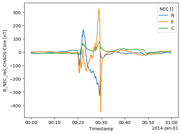
Note that xarray also allows convenient direct plotting like:

ds["B_NEC_res_CHAOS-Core"].plot.line(x="Timestamp");

Access multiple MAG datasets simultaneously

It is possible to fetch data from multiple collections simultaneously. Here we fetch the measurements from Swarm Alpha and Bravo. In the returned data, you can differentiate between them using the “Spacecraft” column.

request = SwarmRequest()
request.set_collection("SW_OPER_MAGA_LR_1B", "SW_OPER_MAGC_LR_1B")
request.set_products(
    measurements=["F", "B_NEC"],
    models=[
        "CHAOS-Core",
    ],
    residuals=True,
    sampling_step="PT10S",
)
data = request.get_between(
    start_time=dt.datetime(2014, 1, 1, 0), end_time=dt.datetime(2014, 1, 1, 1)
)
df = data.as_dataframe(expand=True)
df.head()

	Longitude	Radius	Spacecraft	Latitude	F_res_CHAOS-Core	B_NEC_res_CHAOS-Core_N	B_NEC_res_CHAOS-Core_E	B_NEC_res_CHAOS-Core_C
Timestamp
2014-01-01 00:00:00	-14.116674	6878309.23	A	-1.228938	-6.622418	-9.804910	1.692836	-4.951658
2014-01-01 00:00:10	-14.131424	6878381.18	A	-1.862521	-6.331871	-9.795320	2.583734	-5.481087
2014-01-01 00:00:20	-14.146155	6878452.06	A	-2.496090	-6.063890	-9.799162	2.734860	-5.635835
2014-01-01 00:00:30	-14.160861	6878521.88	A	-3.129644	-5.820963	-9.809455	2.543664	-5.614695
2014-01-01 00:00:40	-14.175534	6878590.62	A	-3.763184	-5.539641	-9.906449	1.942109	-5.710623

df[df["Spacecraft"] == "A"].head()

	Longitude	Radius	Spacecraft	Latitude	F_res_CHAOS-Core	B_NEC_res_CHAOS-Core_N	B_NEC_res_CHAOS-Core_E	B_NEC_res_CHAOS-Core_C
Timestamp
2014-01-01 00:00:00	-14.116674	6878309.23	A	-1.228938	-6.622418	-9.804910	1.692836	-4.951658
2014-01-01 00:00:10	-14.131424	6878381.18	A	-1.862521	-6.331871	-9.795320	2.583734	-5.481087
2014-01-01 00:00:20	-14.146155	6878452.06	A	-2.496090	-6.063890	-9.799162	2.734860	-5.635835
2014-01-01 00:00:30	-14.160861	6878521.88	A	-3.129644	-5.820963	-9.809455	2.543664	-5.614695
2014-01-01 00:00:40	-14.175534	6878590.62	A	-3.763184	-5.539641	-9.906449	1.942109	-5.710623

df[df["Spacecraft"] == "C"].head()

	Longitude	Radius	Spacecraft	Latitude	F_res_CHAOS-Core	B_NEC_res_CHAOS-Core_N	B_NEC_res_CHAOS-Core_E	B_NEC_res_CHAOS-Core_C
Timestamp
2014-01-01 00:00:00	-14.420068	6877665.96	C	5.908082	-10.413440	-10.533725	2.390138	-1.289309
2014-01-01 00:00:10	-14.434576	6877747.64	C	5.274386	-10.000957	-10.283579	2.485700	-1.748991
2014-01-01 00:00:20	-14.449141	6877828.36	C	4.640702	-9.667835	-10.166119	2.401007	-2.174997
2014-01-01 00:00:30	-14.463755	6877908.12	C	4.007030	-9.409666	-10.259289	2.011146	-2.763503
2014-01-01 00:00:40	-14.478412	6877986.90	C	3.373371	-9.142413	-10.333386	1.515452	-3.171075

… or using xarray

ds = data.as_xarray()
ds.where(ds["Spacecraft"] == "A", drop=True)

<xarray.Dataset>
Dimensions:               (Timestamp: 360, NEC: 3)
Coordinates:
  * Timestamp             (Timestamp) datetime64[ns] 2014-01-01 ... 2014-01-0...
  * NEC                   (NEC) <U1 'N' 'E' 'C'
Data variables:
    Spacecraft            (Timestamp) object 'A' 'A' 'A' 'A' ... 'A' 'A' 'A' 'A'
    B_NEC_res_CHAOS-Core  (Timestamp, NEC) float64 -9.805 1.693 ... 3.848 8.99
    Longitude             (Timestamp) float64 -14.12 -14.13 ... 153.6 153.6
    Radius                (Timestamp) float64 6.878e+06 6.878e+06 ... 6.868e+06
    Latitude              (Timestamp) float64 -1.229 -1.863 ... 48.14 48.77
    F_res_CHAOS-Core      (Timestamp) float64 -6.622 -6.332 ... 4.011 3.99
Attributes:
    Sources:         ['SW_OPER_MAGA_LR_1B_20140101T000000_20140101T235959_070...
    MagneticModels:  ["CHAOS-Core = 'CHAOS-Core'(max_degree=20,min_degree=1)"]
    AppliedFilters:  []

xarray.Dataset

• Dimensions:
  • Timestamp: 360
  • NEC: 3
• Coordinates: (2)
  • Timestamp
    (Timestamp)
    datetime64[ns]
    2014-01-01 ... 2014-01-01T00:59:50

    description :

    Time stamp

    array(['2014-01-01T00:00:00.000000000', '2014-01-01T00:00:10.000000000',
           '2014-01-01T00:00:20.000000000', ..., '2014-01-01T00:59:30.000000000',
           '2014-01-01T00:59:40.000000000', '2014-01-01T00:59:50.000000000'],
          dtype='datetime64[ns]')

  • NEC
    (NEC)
    <U1
    'N' 'E' 'C'

    units :

    description :

    NEC frame - North, East, Centre (down)

    array(['N', 'E', 'C'], dtype='<U1')

• Data variables: (6)
  • Spacecraft
    (Timestamp)
    object
    'A' 'A' 'A' 'A' ... 'A' 'A' 'A' 'A'

    units :

    -

    description :

    Spacecraft identifier (values: 'A', 'B', 'C' or '-' if not available).

    array(['A', 'A', 'A', 'A', 'A', 'A', 'A', 'A', 'A', 'A', 'A', 'A', 'A',
           'A', 'A', 'A', 'A', 'A', 'A', 'A', 'A', 'A', 'A', 'A', 'A', 'A',
           'A', 'A', 'A', 'A', 'A', 'A', 'A', 'A', 'A', 'A', 'A', 'A', 'A',
           'A', 'A', 'A', 'A', 'A', 'A', 'A', 'A', 'A', 'A', 'A', 'A', 'A',
           'A', 'A', 'A', 'A', 'A', 'A', 'A', 'A', 'A', 'A', 'A', 'A', 'A',
           'A', 'A', 'A', 'A', 'A', 'A', 'A', 'A', 'A', 'A', 'A', 'A', 'A',
           'A', 'A', 'A', 'A', 'A', 'A', 'A', 'A', 'A', 'A', 'A', 'A', 'A',
           'A', 'A', 'A', 'A', 'A', 'A', 'A', 'A', 'A', 'A', 'A', 'A', 'A',
           'A', 'A', 'A', 'A', 'A', 'A', 'A', 'A', 'A', 'A', 'A', 'A', 'A',
           'A', 'A', 'A', 'A', 'A', 'A', 'A', 'A', 'A', 'A', 'A', 'A', 'A',
           'A', 'A', 'A', 'A', 'A', 'A', 'A', 'A', 'A', 'A', 'A', 'A', 'A',
           'A', 'A', 'A', 'A', 'A', 'A', 'A', 'A', 'A', 'A', 'A', 'A', 'A',
           'A', 'A', 'A', 'A', 'A', 'A', 'A', 'A', 'A', 'A', 'A', 'A', 'A',
           'A', 'A', 'A', 'A', 'A', 'A', 'A', 'A', 'A', 'A', 'A', 'A', 'A',
           'A', 'A', 'A', 'A', 'A', 'A', 'A', 'A', 'A', 'A', 'A', 'A', 'A',
           'A', 'A', 'A', 'A', 'A', 'A', 'A', 'A', 'A', 'A', 'A', 'A', 'A',
           'A', 'A', 'A', 'A', 'A', 'A', 'A', 'A', 'A', 'A', 'A', 'A', 'A',
           'A', 'A', 'A', 'A', 'A', 'A', 'A', 'A', 'A', 'A', 'A', 'A', 'A',
           'A', 'A', 'A', 'A', 'A', 'A', 'A', 'A', 'A', 'A', 'A', 'A', 'A',
           'A', 'A', 'A', 'A', 'A', 'A', 'A', 'A', 'A', 'A', 'A', 'A', 'A',
           'A', 'A', 'A', 'A', 'A', 'A', 'A', 'A', 'A', 'A', 'A', 'A', 'A',
           'A', 'A', 'A', 'A', 'A', 'A', 'A', 'A', 'A', 'A', 'A', 'A', 'A',
           'A', 'A', 'A', 'A', 'A', 'A', 'A', 'A', 'A', 'A', 'A', 'A', 'A',
           'A', 'A', 'A', 'A', 'A', 'A', 'A', 'A', 'A', 'A', 'A', 'A', 'A',
           'A', 'A', 'A', 'A', 'A', 'A', 'A', 'A', 'A', 'A', 'A', 'A', 'A',
           'A', 'A', 'A', 'A', 'A', 'A', 'A', 'A', 'A', 'A', 'A', 'A', 'A',
           'A', 'A', 'A', 'A', 'A', 'A', 'A', 'A', 'A', 'A', 'A', 'A', 'A',
           'A', 'A', 'A', 'A', 'A', 'A', 'A', 'A', 'A'], dtype=object)

  • B_NEC_res_CHAOS-Core
    (Timestamp, NEC)
    float64
    -9.805 1.693 -4.952 ... 3.848 8.99

    units :

    nT

    description :

    Magnetic field vector residual, NEC frame, calculated as a difference of the measurement and value of the CHAOS-Core spherical harmonic model

    array([[-9.80491006,  1.69283596, -4.95165823],
           [-9.79532012,  2.58373387, -5.48108743],
           [-9.79916173,  2.73486005, -5.63583481],
           ...,
           [-5.65857833,  4.31508279,  7.74779816],
           [-7.80581803,  4.27481715,  8.97127872],
           [-8.13059511,  3.84795008,  8.99044822]])

  • Longitude
    (Timestamp)
    float64
    -14.12 -14.13 ... 153.6 153.6

    units :

    deg

    description :

    Position in ITRF - Longitude

    array([-14.1166743, -14.1314243, -14.1461554, -14.1608609, -14.1755342,
           -14.1901685, -14.2047571, -14.2192932, -14.2337699, -14.2481804,
           -14.2625177, -14.2767748, -14.2909444, -14.3050195, -14.3189927,
           -14.3328566, -14.3466037, -14.3602264, -14.3737168, -14.3870671,
           -14.4002693, -14.4133151, -14.4261961, -14.4389038, -14.4514295,
           -14.4637642, -14.4758988, -14.4878238, -14.4995298, -14.5110068,
           -14.5222447, -14.5332332, -14.5439615, -14.5544187, -14.5645933,
           -14.5744739, -14.5840483, -14.5933041, -14.6022285, -14.6108083,
           -14.6190299, -14.6268789, -14.6343409, -14.6414006, -14.6480422,
           -14.6542495, -14.6600055, -14.6652927, -14.6700926, -14.6743864,
           -14.6781542, -14.6813754, -14.6840285, -14.6860912, -14.6875401,
           -14.6883507, -14.6884977, -14.6879543, -14.6866927, -14.6846837,
           -14.6818967, -14.6782997, -14.673859 , -14.6685394, -14.6623038,
           -14.6551131, -14.6469263, -14.6377003, -14.6273894, -14.6159457,
           -14.6033184, -14.589454 , -14.5742958, -14.557784 , -14.539855 ,
           -14.5204415, -14.4994721, -14.476871 , -14.4525575, -14.4264457,
           -14.3984442, -14.3684554, -14.3363752, -14.3020922, -14.2654873,
           -14.2264328, -14.1847917, -14.1404169, -14.0931501, -14.0428207,
           -13.989245 , -13.9322242, -13.8715433, -13.8069696, -13.73825  ,
           -13.6651097, -13.5872493, -13.5043418, -13.41603  , -13.3219222,
    ...
           154.3456616, 154.3325292, 154.3192466, 154.3058218, 154.2922629,
           154.2785777, 154.2647737, 154.2508587, 154.23684  , 154.222725 ,
           154.2085209, 154.1942349, 154.1798741, 154.1654455, 154.1509559,
           154.1364123, 154.1218215, 154.1071902, 154.0925253, 154.0778333,
           154.063121 , 154.048395 , 154.033662 , 154.0189287, 154.0042015,
           153.9894873, 153.9747926, 153.9601241, 153.9454886, 153.9308927,
           153.9163432, 153.901847 , 153.8874109, 153.8730419, 153.8587469,
           153.8445331, 153.8304075, 153.8163774, 153.8024502, 153.7886334,
           153.7749344, 153.761361 , 153.7479209, 153.7346221, 153.7214728,
           153.7084812, 153.6956557, 153.6830049, 153.6705376, 153.6582628,
           153.6461898, 153.634328 , 153.622687 , 153.6112768, 153.6001075,
           153.5891898, 153.5785343, 153.5681521, 153.5580546, 153.5482537,
           153.5387614, 153.5295904, 153.5207534, 153.5122638, 153.5041356,
           153.496383 , 153.4890208, 153.4820643, 153.4755295, 153.4694328,
           153.4637914, 153.4586231, 153.4539463, 153.4497804, 153.4461453,
           153.443062 , 153.4405521, 153.4386383, 153.4373443, 153.4366949,
           153.4367157, 153.4374339, 153.4388777, 153.4410767, 153.4440618,
           153.4478657, 153.4525224, 153.4580678, 153.4645395, 153.4719771,
           153.4804224, 153.4899192, 153.5005138, 153.5122551, 153.5251946,
           153.5393868, 153.5548894, 153.5717634, 153.5900733, 153.6098879])

  • Radius
    (Timestamp)
    float64
    6.878e+06 6.878e+06 ... 6.868e+06

    units :

    m

    description :

    Position in ITRF - Radius

    array([6878309.23, 6878381.18, 6878452.06, 6878521.88, 6878590.62,
           6878658.28, 6878724.85, 6878790.33, 6878854.71, 6878917.98,
           6878980.14, 6879041.19, 6879101.13, 6879159.94, 6879217.64,
           6879274.21, 6879329.65, 6879383.96, 6879437.15, 6879489.2 ,
           6879540.13, 6879589.92, 6879638.58, 6879686.12, 6879732.52,
           6879777.8 , 6879821.96, 6879864.99, 6879906.9 , 6879947.69,
           6879987.37, 6880025.93, 6880063.39, 6880099.75, 6880135.01,
           6880169.17, 6880202.25, 6880234.24, 6880265.16, 6880295.  ,
           6880323.78, 6880351.5 , 6880378.17, 6880403.8 , 6880428.39,
           6880451.95, 6880474.49, 6880496.01, 6880516.54, 6880536.07,
           6880554.61, 6880572.18, 6880588.78, 6880604.42, 6880619.12,
           6880632.88, 6880645.71, 6880657.63, 6880668.64, 6880678.76,
           6880687.99, 6880696.36, 6880703.86, 6880710.51, 6880716.33,
           6880721.32, 6880725.5 , 6880728.88, 6880731.47, 6880733.28,
           6880734.34, 6880734.64, 6880734.21, 6880733.05, 6880731.18,
           6880728.61, 6880725.36, 6880721.44, 6880716.86, 6880711.63,
           6880705.78, 6880699.3 , 6880692.23, 6880684.56, 6880676.31,
           6880667.5 , 6880658.14, 6880648.24, 6880637.81, 6880626.88,
           6880615.45, 6880603.54, 6880591.15, 6880578.3 , 6880565.02,
           6880551.29, 6880537.16, 6880522.61, 6880507.67, 6880492.36,
    ...
           6875648.21, 6875587.21, 6875525.54, 6875463.21, 6875400.22,
           6875336.57, 6875272.26, 6875207.3 , 6875141.68, 6875075.42,
           6875008.52, 6874940.98, 6874872.8 , 6874804.  , 6874734.58,
           6874664.55, 6874593.9 , 6874522.66, 6874450.83, 6874378.4 ,
           6874305.41, 6874231.84, 6874157.71, 6874083.03, 6874007.82,
           6873932.07, 6873855.8 , 6873779.02, 6873701.74, 6873623.97,
           6873545.73, 6873467.02, 6873387.86, 6873308.26, 6873228.24,
           6873147.8 , 6873066.96, 6872985.74, 6872904.15, 6872822.2 ,
           6872739.91, 6872657.3 , 6872574.37, 6872491.16, 6872407.66,
           6872323.9 , 6872239.9 , 6872155.67, 6872071.23, 6871986.6 ,
           6871901.79, 6871816.82, 6871731.71, 6871646.48, 6871561.14,
           6871475.72, 6871390.23, 6871304.7 , 6871219.15, 6871133.59,
           6871048.04, 6870962.54, 6870877.08, 6870791.71, 6870706.43,
           6870621.28, 6870536.27, 6870451.42, 6870366.75, 6870282.3 ,
           6870198.07, 6870114.09, 6870030.39, 6869946.98, 6869863.89,
           6869781.14, 6869698.75, 6869616.75, 6869535.15, 6869453.98,
           6869373.26, 6869293.01, 6869213.27, 6869134.03, 6869055.34,
           6868977.21, 6868899.67, 6868822.73, 6868746.41, 6868670.75,
           6868595.76, 6868521.47, 6868447.89, 6868375.05, 6868302.96,
           6868231.66, 6868161.16, 6868091.48, 6868022.65, 6867954.68])

  • Latitude
    (Timestamp)
    float64
    -1.229 -1.863 ... 48.14 48.77

    units :

    deg

    description :

    Position in ITRF - Latitude

    array([ -1.2289378,  -1.8625209,  -2.4960899,  -3.1296444,  -3.7631844,
            -4.3967096,  -5.03022  ,  -5.6637153,  -6.2971954,  -6.9306601,
            -7.5641093,  -8.1975429,  -8.8309607,  -9.4643624, -10.097748 ,
           -10.7311174, -11.3644703, -11.9978066, -12.6311262, -13.2644288,
           -13.8977144, -14.5309828, -15.1642339, -15.7974674, -16.4306832,
           -17.0638811, -17.6970611, -18.3302228, -18.9633662, -19.5964911,
           -20.2295972, -20.8626845, -21.4957527, -22.1288017, -22.7618311,
           -23.394841 , -24.027831 , -24.6608009, -25.2937505, -25.9266797,
           -26.5595881, -27.1924756, -27.8253419, -28.4581867, -29.0910097,
           -29.7238108, -30.3565896, -30.9893458, -31.6220792, -32.2547893,
           -32.8874759, -33.5201386, -34.1527771, -34.7853909, -35.4179797,
           -36.0505431, -36.6830805, -37.3155916, -37.9480759, -38.5805328,
           -39.2129618, -39.8453623, -40.4777338, -41.1100755, -41.7423869,
           -42.3746672, -43.0069157, -43.6391316, -44.271314 , -44.903462 ,
           -45.5355747, -46.1676512, -46.7996902, -47.4316908, -48.0636516,
           -48.6955714, -49.3274489, -49.9592824, -50.5910706, -51.2228116,
           -51.8545038, -52.4861451, -53.1177335, -53.7492668, -54.3807426,
           -55.0121584, -55.6435114, -56.2747985, -56.9060167, -57.5371623,
           -58.1682317, -58.7992208, -59.4301252, -60.06094  , -60.69166  ,
           -61.3222795, -61.9527922, -62.5831914, -63.2134696, -63.8436184,
    ...
           -14.0397279, -13.4057211, -12.7716953, -12.1376508, -11.5035876,
           -10.8695063, -10.2354069,  -9.6012897,  -8.967155 ,  -8.333003 ,
            -7.6988341,  -7.0646483,  -6.4304461,  -5.7962276,  -5.161993 ,
            -4.5277427,  -3.8934769,  -3.2591959,  -2.6248998,  -1.990589 ,
            -1.3562637,  -0.7219241,  -0.0875706,   0.5467966,   1.1811773,
             1.8155712,   2.449978 ,   3.0843975,   3.7188294,   4.3532734,
             4.9877293,   5.6221967,   6.2566755,   6.8911653,   7.5256657,
             8.1601767,   8.7946978,   9.4292288,  10.0637693,  10.6983191,
            11.3328779,  11.9674454,  12.6020212,  13.2366051,  13.8711967,
            14.5057958,  15.1404019,  15.7750149,  16.4096342,  17.0442597,
            17.6788909,  18.3135275,  18.9481692,  19.5828155,  20.2174661,
            20.8521207,  21.4867788,  22.1214401,  22.7561042,  23.3907706,
            24.025439 ,  24.6601089,  25.2947799,  25.9294516,  26.5641235,
            27.1987952,  27.8334661,  28.4681359,  29.102804 ,  29.7374699,
            30.3721332,  31.0067932,  31.6414495,  32.2761015,  32.9107485,
            33.5453901,  34.1800256,  34.8146544,  35.4492757,  36.083889 ,
            36.7184936,  37.3530887,  37.9876736,  38.6222475,  39.2568096,
            39.891359 ,  40.525895 ,  41.1604165,  41.7949226,  42.4294124,
            43.0638848,  43.6983388,  44.3327731,  44.9671867,  45.6015782,
            46.2359464,  46.87029  ,  47.5046074,  48.1388971,  48.7731577])

  • F_res_CHAOS-Core
    (Timestamp)
    float64
    -6.622 -6.332 -6.064 ... 4.011 3.99

    units :

    nT

    description :

    Magnetic field intensity residual, calculated as a difference of the measurement and value of the CHAOS-Core spherical harmonic model

    array([ -6.62241801,  -6.33187125,  -6.0638898 ,  -5.82096342,
            -5.53964121,  -5.23397026,  -4.91309535,  -4.60323914,
            -4.22753676,  -4.08447563,  -3.82756674,  -3.56792123,
            -3.29149433,  -3.02207408,  -2.74507316,  -2.4488211 ,
            -2.14816538,  -1.83137593,  -1.51410345,  -1.20151099,
            -0.91083694,  -0.620005  ,  -0.34547901,  -0.06979156,
             0.17428986,   0.40611449,   0.6314765 ,   0.84878474,
             1.06956556,   1.28231328,   1.51343817,   1.75315247,
             1.99143   ,   2.23493703,   2.48367576,   2.72457943,
             2.9703334 ,   3.20528466,   3.42179495,   3.63914629,
             3.84096842,   4.03843078,   4.22826593,   4.42044693,
             4.58311622,   4.74401038,   4.91556718,   5.07501769,
             5.22728957,   5.37924472,   5.53677327,   5.70090907,
             5.89454047,   6.10370395,   6.31390265,   6.51878299,
             6.72021663,   6.89969708,   7.05335849,   7.18851978,
             7.30797017,   7.42394951,   7.54198983,   7.68240446,
             7.8471169 ,   8.02841887,   8.24561372,   8.47910942,
             8.72270858,   8.97757811,   9.22497908,   9.47432978,
             9.70693634,   9.9177923 ,  10.11840788,  10.29094956,
            10.45013548,  10.5974559 ,  10.75987108,  10.90408902,
    ...
           -11.49495788, -11.1879719 , -11.19547779, -11.57081478,
           -12.31362088, -13.41461884, -14.93282896, -16.7692074 ,
           -18.81238541, -20.90532131, -22.89119778, -24.54347032,
           -25.59703712, -25.81844717, -25.10622745, -23.49213392,
           -21.13905378, -18.33606471, -15.38638051, -12.57363263,
           -10.09695736,  -8.06390827,  -6.5437512 ,  -5.49207406,
            -4.85223405,  -4.52991342,  -4.43906796,  -4.51856228,
            -4.67806122,  -4.85127951,  -5.01743957,  -5.18094524,
            -5.36202706,  -5.60036533,  -5.84073174,  -6.03342947,
            -6.16021735,  -6.26219807,  -6.33216977,  -6.35166263,
            -6.2850046 ,  -6.16420921,  -5.97436883,  -5.70981916,
            -5.44376112,  -5.18869119,  -5.01387281,  -4.89499068,
            -4.88445565,  -4.95893851,  -5.10251186,  -5.28088137,
            -5.50990837,  -5.6949186 ,  -5.74651547,  -5.62997448,
            -5.40495271,  -5.08460347,  -4.69022738,  -4.22126933,
            -3.7370415 ,  -3.22192136,  -2.67739507,  -2.14371935,
            -1.58337728,  -0.97901484,  -0.32935864,   0.29385849,
             0.87343232,   1.35266389,   1.74707834,   2.04182371,
             2.29576754,   2.55026647,   2.86013012,   3.18523201,
             3.52738804,   3.84880579,   4.01115736,   3.99019678])

• Indexes: (2)
  • Timestamp
    PandasIndex

    PandasIndex(DatetimeIndex(['2014-01-01 00:00:00', '2014-01-01 00:00:10',
                   '2014-01-01 00:00:20', '2014-01-01 00:00:30',
                   '2014-01-01 00:00:40', '2014-01-01 00:00:50',
                   '2014-01-01 00:01:00', '2014-01-01 00:01:10',
                   '2014-01-01 00:01:20', '2014-01-01 00:01:30',
                   ...
                   '2014-01-01 00:58:20', '2014-01-01 00:58:30',
                   '2014-01-01 00:58:40', '2014-01-01 00:58:50',
                   '2014-01-01 00:59:00', '2014-01-01 00:59:10',
                   '2014-01-01 00:59:20', '2014-01-01 00:59:30',
                   '2014-01-01 00:59:40', '2014-01-01 00:59:50'],
                  dtype='datetime64[ns]', name='Timestamp', length=360, freq=None))

  • NEC
    PandasIndex

    PandasIndex(Index(['N', 'E', 'C'], dtype='object', name='NEC'))

• Attributes: (3)

  Sources :

  ['SW_OPER_MAGA_LR_1B_20140101T000000_20140101T235959_0701_MDR_MAG_LR', 'SW_OPER_MAGC_LR_1B_20140101T000000_20140101T235959_0701_MDR_MAG_LR', 'SW_OPER_MCO_SHA_2X_19970101T000000_20260206T235959_0805']

  MagneticModels :

  ["CHAOS-Core = 'CHAOS-Core'(max_degree=20,min_degree=1)"]

  AppliedFilters :

  []