TECxTMS_2F (Total electron content)#
Abstract: Access to the total electric contents (level 2 product).
%load_ext watermark
%watermark -i -v -p viresclient,pandas,xarray,matplotlib
Python implementation: CPython
Python version       : 3.11.6
IPython version      : 8.18.0

viresclient: 0.15.0
pandas     : 2.1.3
xarray     : 2023.12.0
matplotlib : 3.8.2
from viresclient import SwarmRequest
import datetime as dt
import numpy as np
import pandas as pd
import matplotlib.pyplot as plt

request = SwarmRequest()
TECxTMS_2F product information#
Derived total electron content (TEC).
Documentation:
Check what “TEC” data variables are available#
request.available_collections("IPD", details=False)
{'IPD': ['SW_OPER_IPDAIRR_2F', 'SW_OPER_IPDBIRR_2F', 'SW_OPER_IPDCIRR_2F']}
request.available_measurements("TEC")
['GPS_Position',
 'LEO_Position',
 'PRN',
 'L1',
 'L2',
 'P1',
 'P2',
 'S1',
 'S2',
 'Elevation_Angle',
 'Absolute_VTEC',
 'Absolute_STEC',
 'Relative_STEC',
 'Relative_STEC_RMS',
 'DCB',
 'DCB_Error']
Fetch one day of TEC data#
request.set_collection("SW_OPER_TECATMS_2F")
request.set_products(measurements=request.available_measurements("TEC"))
data = request.get_between(dt.datetime(2014, 1, 1), dt.datetime(2014, 1, 2))
Loading as pandas#
df = data.as_dataframe()
df.head()
| Radius | Spacecraft | L2 | Absolute_STEC | Latitude | Absolute_VTEC | DCB | S1 | Relative_STEC | L1 | Longitude | PRN | P1 | DCB_Error | S2 | Relative_STEC_RMS | Elevation_Angle | GPS_Position | P2 | LEO_Position | |
|---|---|---|---|---|---|---|---|---|---|---|---|---|---|---|---|---|---|---|---|---|
| Timestamp | ||||||||||||||||||||
| 2014-01-01 00:00:04 | 6.878338e+06 | A | -6.261989e+06 | 16.429938 | -1.482419 | 10.894886 | -11.446853 | 36.83 | 24.041127 | -6.261986e+06 | -14.122572 | 15 | 2.182913e+07 | 0.832346 | 36.83 | 0.555675 | 39.683333 | [22448765.690377887, 5421379.431197803, -13409... | 2.182914e+07 | [6668214.552999999, -1677732.678, -177943.998] |
| 2014-01-01 00:00:04 | 6.878338e+06 | A | -1.466568e+07 | 16.456409 | -1.482419 | 10.461554 | -11.446853 | 34.75 | 22.754795 | -1.466568e+07 | -14.122572 | 18 | 2.135749e+07 | 0.832346 | 34.75 | 0.488000 | 37.478137 | [16113499.491062254, -16306172.004347403, -126... | 2.135749e+07 | [6668214.552999999, -1677732.678, -177943.998] |
| 2014-01-01 00:00:04 | 6.878338e+06 | A | -5.455454e+06 | 20.434286 | -1.482419 | 9.529846 | -11.446853 | 30.90 | 15.585271 | -5.455452e+06 | -14.122572 | 22 | 2.277638e+07 | 0.832346 | 30.90 | 1.313984 | 24.681787 | [10823457.339250825, -24014739.352816023, -248... | 2.277638e+07 | [6668214.552999999, -1677732.678, -177943.998] |
| 2014-01-01 00:00:04 | 6.878338e+06 | A | -3.402821e+06 | 20.085094 | -1.482419 | 9.357587 | -11.446853 | 29.87 | 52.291341 | -3.402816e+06 | -14.122572 | 24 | 2.298846e+07 | 0.832346 | 29.87 | 0.899036 | 24.647445 | [20631539.59055339, 13441368.439225309, 100505... | 2.298847e+07 | [6668214.552999999, -1677732.678, -177943.998] |
| 2014-01-01 00:00:04 | 6.878338e+06 | A | -2.285986e+06 | 15.676947 | -1.482419 | 8.597559 | -11.446853 | 30.88 | 52.672067 | -2.285981e+06 | -14.122572 | 25 | 2.229899e+07 | 0.832346 | 30.88 | 0.546729 | 30.753636 | [16637723.905075422, -10692759.977004562, 1761... | 2.229900e+07 | [6668214.552999999, -1677732.678, -177943.998] |
NB: The time interval is not always the same:
times = df.index
np.unique(np.sort(np.diff(times.to_pydatetime())))
array([datetime.timedelta(0), datetime.timedelta(seconds=10)],
      dtype=object)
len(df), 60 * 60 * 24
(49738, 86400)
Loading and plotting as xarray#
ds = data.as_xarray()
ds
<xarray.Dataset>
Dimensions:            (Timestamp: 49738, WGS84: 3)
Coordinates:
  * Timestamp          (Timestamp) datetime64[ns] 2014-01-01T00:00:04 ... 201...
  * WGS84              (WGS84) <U1 'X' 'Y' 'Z'
Data variables: (12/20)
    Spacecraft         (Timestamp) object 'A' 'A' 'A' 'A' ... 'A' 'A' 'A' 'A'
    Radius             (Timestamp) float64 6.878e+06 6.878e+06 ... 6.88e+06
    L2                 (Timestamp) float64 -6.262e+06 -1.467e+07 ... -3.41e+06
    Absolute_STEC      (Timestamp) float64 16.43 16.46 20.43 ... 10.77 10.78
    Latitude           (Timestamp) float64 -1.482 -1.482 -1.482 ... -81.7 -81.7
    Absolute_VTEC      (Timestamp) float64 10.89 10.46 9.53 ... 8.365 7.912
    ...                 ...
    S2                 (Timestamp) float64 36.83 34.75 30.9 ... 23.03 37.73 37.5
    Relative_STEC_RMS  (Timestamp) float64 0.5557 0.488 1.314 ... 0.6458 3.041
    Elevation_Angle    (Timestamp) float64 39.68 37.48 24.68 ... 49.64 45.71
    GPS_Position       (Timestamp, WGS84) float64 2.245e+07 ... -2.111e+07
    P2                 (Timestamp) float64 2.183e+07 2.136e+07 ... 2.171e+07
    LEO_Position       (Timestamp, WGS84) float64 6.668e+06 ... -6.808e+06
Attributes:
    Sources:         ['SW_OPER_TECATMS_2F_20140101T000000_20140101T235959_0401']
    MagneticModels:  []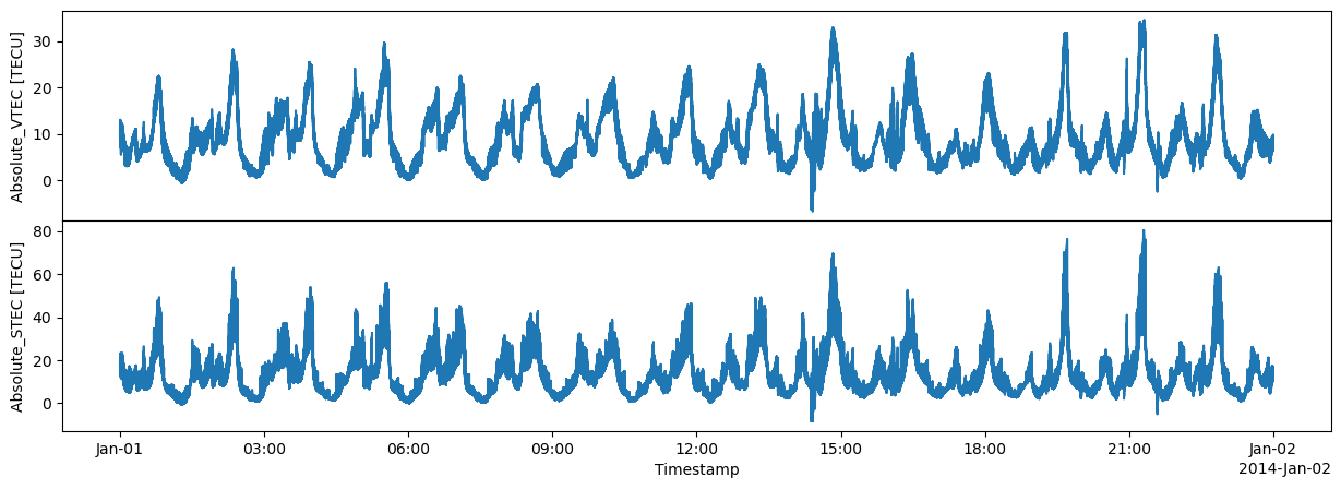
AppliedFilters: []fig, axes = plt.subplots(nrows=2, ncols=1, figsize=(15, 5), sharex=True)
ds["Absolute_VTEC"].plot.line(x="Timestamp", ax=axes[0])
ds["Absolute_STEC"].plot.line(x="Timestamp", ax=axes[1])
fig.subplots_adjust(hspace=0)