EFIxIDM (Ion drifts & effective masses)#
Abstract: Access to the
EFIxIDMproducts from the SLIDEM project.
Documentation:
Additional examples:
# Display important package versions used
%load_ext watermark
%watermark -i -v -p viresclient,pandas,xarray,matplotlib
Python implementation: CPython
Python version       : 3.11.6
IPython version      : 8.18.0

viresclient: 0.15.0
pandas     : 2.1.3
xarray     : 2023.12.0
matplotlib : 3.8.2
import datetime as dt
import matplotlib as mpl
import matplotlib.pyplot as plt
import numpy as np
import xarray as xr

# Control the HTML display of the datasets
xr.set_options(
    display_expand_attrs=False, display_expand_coords=True, display_expand_data=True
)

from viresclient import SwarmRequest
request = SwarmRequest()
What data is available?#
request.available_collections("EFI_IDM", details=False)
{'EFI_IDM': ['SW_PREL_EFIAIDM_2_', 'SW_PREL_EFIBIDM_2_', 'SW_PREL_EFICIDM_2_']}
print(request.available_measurements("EFI_IDM"))
['Latitude_GD', 'Longitude_GD', 'Height_GD', 'Radius_GC', 'Latitude_QD', 'MLT_QD', 'V_sat_nec', 'M_i_eff', 'M_i_eff_err', 'M_i_eff_Flags', 'M_i_eff_tbt_model', 'V_i', 'V_i_err', 'V_i_Flags', 'V_i_raw', 'N_i', 'N_i_err', 'N_i_Flags', 'A_fp', 'R_p', 'T_e', 'Phi_sc']
Notes for the listed available variables:
idm_vars = [
    # Positional information in geodetic (GD) and geocentric (GC) frames
    #  redundant with VirES variables Latitude, Longitude, Radius (in geocentric frame)
    "Latitude_GD",
    "Longitude_GD",
    "Height_GD",
    "Radius_GC",
    # Quasi-dipole magnetic latitude and local time
    #  redundant with VirES auxiliaries, QDLat & MLT
    "Latitude_QD",
    "MLT_QD",
    # Satellite velocity in NEC frame
    "V_sat_nec",
    # Estimated ion effective mass, uncertainty, and validity flags
    "M_i_eff",
    "M_i_eff_err",
    "M_i_eff_Flags",
    # Effective masses from ruhlik et al. (2015) topside empirical model
    "M_i_eff_tbt_model",
    # Along-track ion drift velocity, uncertainty, validity flags, and velocity without detrending
    "V_i",
    "V_i_err",
    "V_i_Flags",
    "V_i_raw",
    # Ion density, uncertainty, and validity flags
    "N_i",
    "N_i_err",
    "N_i_Flags",
    # Modified-OML faceplate area, and Langmuir spherical probe radius
    "A_fp",
    "R_p",
    # Electron temperature, and spacecraft floating potential
    "T_e",
    "Phi_sc",
]
Fetching and plotting data#
start = dt.datetime(2016, 1, 2)
end = dt.datetime(2016, 1, 3)

request = SwarmRequest()
request.set_collection("SW_PREL_EFIAIDM_2_")
request.set_products(
    measurements=idm_vars, auxiliaries=["OrbitNumber", "OrbitDirection", "MLT"]
)
data = request.get_between(start, end)
Data can be loaded as either a pandas dataframe or a xarray dataset.
df = data.as_dataframe()
df.head()
| M_i_eff_err | V_i_raw | Latitude | N_i_Flags | M_i_eff | MLT | Latitude_GD | V_i_err | Spacecraft | Longitude | ... | Radius_GC | Latitude_QD | Radius | MLT_QD | N_i_err | OrbitDirection | M_i_eff_Flags | T_e | V_i_Flags | Longitude_GD | |
|---|---|---|---|---|---|---|---|---|---|---|---|---|---|---|---|---|---|---|---|---|---|
| Timestamp | |||||||||||||||||||||
| 2016-01-02 00:00:00.196999936 | -1.0 | -100000.0 | 31.751028 | 1 | -1.0 | 17.155861 | 31.912074 | -1.0 | A | -95.369735 | ... | 6.821611e+06 | 41.452417 | 6.822807e+06 | 17.699699 | -1.0 | 1 | 1 | 2660.305569 | 65537 | -95.369735 |
| 2016-01-02 00:00:00.696000000 | -1.0 | -100000.0 | 31.783018 | 1 | -1.0 | 17.155920 | 31.944152 | -1.0 | A | -95.369768 | ... | 6.821616e+06 | 41.484162 | 6.822801e+06 | 17.699779 | -1.0 | 1 | 1 | 2640.667985 | 65537 | -95.369768 |
| 2016-01-02 00:00:01.196999936 | -1.0 | -100000.0 | 31.815135 | 1 | -1.0 | 17.155981 | 31.976359 | -1.0 | A | -95.369800 | ... | 6.821621e+06 | 41.516033 | 6.822795e+06 | 17.699859 | -1.0 | 1 | 1 | 2629.307430 | 65537 | -95.369800 |
| 2016-01-02 00:00:01.696000000 | -1.0 | -100000.0 | 31.847124 | 1 | -1.0 | 17.156040 | 32.008436 | -1.0 | A | -95.369831 | ... | 6.821626e+06 | 41.547775 | 6.822789e+06 | 17.699939 | -1.0 | 1 | 1 | 2626.466513 | 65537 | -95.369831 |
| 2016-01-02 00:00:02.196999936 | -1.0 | -100000.0 | 31.879242 | 1 | -1.0 | 17.156099 | 32.040643 | -1.0 | A | -95.369860 | ... | 6.821630e+06 | 41.579643 | 6.822783e+06 | 17.700020 | -1.0 | 1 | 1 | 2645.862873 | 65537 | -95.369860 |
5 rows × 29 columns
ds = data.as_xarray()
ds
<xarray.Dataset>
Dimensions:            (Timestamp: 171434, V_sat_nec_dim1: 3)
Coordinates:
  * Timestamp          (Timestamp) datetime64[ns] 2016-01-02T00:00:00.1969999...
Dimensions without coordinates: V_sat_nec_dim1
Data variables: (12/29)
    Spacecraft         (Timestamp) object 'A' 'A' 'A' 'A' ... 'A' 'A' 'A' 'A'
    M_i_eff_err        (Timestamp) float64 -1.0 -1.0 -1.0 ... -1.0 -1.0 -1.0
    V_i_raw            (Timestamp) float64 -1e+05 -1e+05 ... -1e+05 -1e+05
    Latitude           (Timestamp) float64 31.75 31.78 31.82 ... 8.711 8.679
    N_i_Flags          (Timestamp) uint32 1 1 1 1 1 1 1 1 1 ... 1 1 1 1 1 1 1 1
    M_i_eff            (Timestamp) float64 -1.0 -1.0 -1.0 ... -1.0 -1.0 -1.0
    ...                 ...
    N_i_err            (Timestamp) float64 -1.0 -1.0 -1.0 ... -1.0 -1.0 -1.0
    OrbitDirection     (Timestamp) int8 1 1 1 1 1 1 1 1 ... -1 -1 -1 -1 -1 -1 -1
    M_i_eff_Flags      (Timestamp) uint32 1 1 1 1 1 1 1 1 1 ... 1 1 1 1 1 1 1 1
    T_e                (Timestamp) float64 2.66e+03 2.641e+03 ... 1.73e+03
    V_i_Flags          (Timestamp) uint32 65537 65537 65537 ... 65537 65537
    Longitude_GD       (Timestamp) float64 -95.37 -95.37 -95.37 ... 81.23 81.23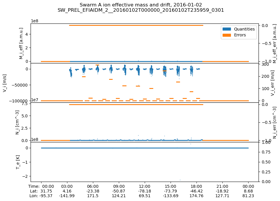
Attributes: (3)An initial preview of the data:
fig, axes = plt.subplots(nrows=4, sharex=True, figsize=(10, 7))
axes_r = [ax.twinx() for ax in axes]
# Plot quantity (left axis) and error (right axis) for each quantity
ds.plot.scatter(x="Timestamp", y="M_i_eff", ax=axes[0], s=1, linewidths=0)
ds.plot.scatter(x="Timestamp", y="M_i_eff_err", ax=axes_r[0], s=0.1, color="tab:orange")
ds.plot.scatter(x="Timestamp", y="V_i", ax=axes[1], s=1, linewidths=0)
ds.plot.scatter(x="Timestamp", y="V_i_err", ax=axes_r[1], s=0.1, color="tab:orange")
ds.plot.scatter(x="Timestamp", y="N_i", ax=axes[2], s=1, linewidths=0)
ds.plot.scatter(x="Timestamp", y="N_i_err", ax=axes_r[2], s=0.1, color="tab:orange")
ds.plot.scatter(x="Timestamp", y="T_e", ax=axes[3], s=1, linewidths=0)
fig.subplots_adjust(hspace=0)

# Add legend to identify each side
blue = mpl.patches.Patch(color="tab:blue", label="Quantities")
orange = mpl.patches.Patch(color="tab:orange", label="Errors")
axes[0].legend(handles=[blue, orange])

# # Generate additional ticklabels for x-axis
# Use time xticks to get dataset vars at those xticks
locx = axes[-1].get_xticks()
times = mpl.dates.num2date(locx)
times = [t.replace(tzinfo=None) for t in times]
_ds_xticks = ds.reindex({"Timestamp": times}, method="nearest")
# Build ticklabels from dataset vars
xticklabels = np.stack(
    [
        _ds_xticks["Timestamp"].dt.strftime("%H:%M").values,
        np.round(_ds_xticks["Latitude"].values, 2).astype(str),
        np.round(_ds_xticks["Longitude"].values, 2).astype(str),
    ]
)
xticklabels = ["\n".join(row) for row in xticklabels.T]
# Add labels to first xtick
_xt0 = xticklabels[0].split("\n")
xticklabels[0] = f"Time:  {_xt0[0]}\nLat:  {_xt0[1]}\nLon: {_xt0[2]}"
axes[-1].set_xticks(axes[-1].get_xticks())
axes[-1].set_xticklabels(xticklabels)
axes[-1].set_xlabel("")
# Adjust title
sources = "\n".join([i for i in ds.attrs["Sources"] if "IDM" in i])
title = "".join(
    [
        f"Swarm {ds['Spacecraft'].data[0]} ion effective mass and drift, ",
        ds["Timestamp"].dt.date.data[0].isoformat(),
        f"\n{sources}",
    ]
)
fig.suptitle(title);