AUX_OBS Ground Observatory Data

Abstract: We Demonstrate geomagnetic ground observatory data access through VirES - this is the AUX_OBS product distributed by BGS to support the Swarm mission, and contains data from INTERMAGNET and the World Data Centre (WDC) for Geomagnetism. Data are available as three collections: 1 second and 1 minute cadences (INTERMAGNET definitive & quasi-definitive data), as well as specially derived hourly means over the past century (WDC).

See also:

• https://book.magneticearth.org/geomag-obs-models/01a_visualising-geomagnetic-observatory-data

About the data

The data are also available from the BGS FTP server (ftp.nerc-murchison.ac.uk/geomag/Swarm/AUX_OBS/). If that is more useful to you, you can refer to this older notebook demonstration of access to the FTP server.

Please note the data are under different usage terms than the Swarm data:

• If you use the 1-second or 1-minute data, please refer to the INTERMAGNET data conditions

• If you use the 1-hour data, please also refer to the WDC usage rules and cite the article about the preparation of these data:
  Macmillan, S., Olsen, N. Observatory data and the Swarm mission. Earth Planet Sp 65, 15 (2013). https://doi.org/10.5047/eps.2013.07.011

Caution: The magnetic vector components have been rotated into the geocentric (NEC) frame rather than the geodetic frame, so that they are consistent with the Swarm data. This is in contrast with the data provided directly from observatories.

# Display important package versions used
%load_ext watermark
%watermark -i -v -p viresclient,pandas,xarray,matplotlib

Python implementation: CPython
Python version       : 3.11.6
IPython version      : 8.18.0

viresclient: 0.12.0
pandas     : 2.1.3
xarray     : 2023.12.0
matplotlib : 3.8.2

from viresclient import SwarmRequest
import matplotlib.pyplot as plt

Organisation of data in VirES

AUX_OBS collection types

Data are organised into AUX_OBSH (hour), AUX_OBSM (minute), AUX_OBSS (second) types. For example, to access the hourly data, use the collection name SW_OPER_AUX_OBSH2_.

request = SwarmRequest()
print(request.available_collections("AUX_OBSH", details=False))
print(request.available_collections("AUX_OBSM", details=False))
print(request.available_collections("AUX_OBSS", details=False))

{'AUX_OBSH': ['SW_OPER_AUX_OBSH2_']}
{'AUX_OBSM': ['SW_OPER_AUX_OBSM2_']}
{'AUX_OBSS': ['SW_OPER_AUX_OBSS2_']}

Within each collection, the following variables are available:

print(request.available_measurements("SW_OPER_AUX_OBSH2_"))
print(request.available_measurements("SW_OPER_AUX_OBSM2_"))
print(request.available_measurements("SW_OPER_AUX_OBSS2_"))

['B_NEC', 'F', 'IAGA_code', 'Quality', 'ObsIndex']
['B_NEC', 'F', 'IAGA_code', 'Quality']
['B_NEC', 'F', 'IAGA_code', 'Quality']

• B_NEC and F are the magnetic field vector and intensity

• IAGA_code gives the official three-letter IAGA codes that identify each observatory

• Quality is either “D” or “Q” to indicate whether data is definitive (D) or quasi-definitive (Q)

• ObsIndex is an increasing integer (0, 1, 2…) attached to the hourly data - this indicates a change in the observatory (e.g. of precise location) while the 3-letter IAGA code remained the same

Data can be requested similarly to Swarm MAG products

Note that the IAGA_code variable is necessary in order to distinguish records from each observatory

Note that there is a special message issued regarding the data terms

Let’s fetch all the variables available within the 1-minute data, from two days:

request = SwarmRequest()
request.set_collection("SW_OPER_AUX_OBSM2_")
request.set_products(["IAGA_code", "B_NEC", "F", "Quality"])
data = request.get_between("2016-01-01", "2016-01-03")
ds = data.as_xarray()
ds

Accessing INTERMAGNET and/or WDC data
Check usage terms at ftp://ftp.nerc-murchison.ac.uk/geomag/Swarm/AUX_OBS/minute/README

<xarray.Dataset>
Dimensions:    (Timestamp: 295200, NEC: 3)
Coordinates:
  * Timestamp  (Timestamp) datetime64[ns] 2016-01-01 ... 2016-01-02T23:59:00
  * NEC        (NEC) <U1 'N' 'E' 'C'
Data variables:
    Latitude   (Timestamp) float64 18.5 68.23 -13.73 ... -22.26 47.74 53.56
    Quality    (Timestamp) <U1 'D' 'D' 'D' 'Q' 'D' 'D' ... 'D' 'D' 'Q' 'D' 'D'
    Longitude  (Timestamp) float64 72.87 18.82 171.8 58.6 ... 316.4 15.86 9.073
    IAGA_code  (Timestamp) <U3 'ABG' 'ABK' 'API' 'ARS' ... 'VSS' 'WIC' 'WNG'
    Radius     (Timestamp) float64 6.376e+06 6.36e+06 ... 6.367e+06 6.364e+06
    B_NEC      (Timestamp, NEC) float64 3.804e+04 197.1 ... 764.8 4.623e+04
    F          (Timestamp) float64 4.297e+04 5.33e+04 ... 4.85e+04 4.962e+04
Attributes:
    Sources:         ['SW_OPER_AUX_OBSM2__20160101T000000_20160101T235959_010...
    MagneticModels:  []
    AppliedFilters:  []

xarray.Dataset

• Dimensions:
  • Timestamp: 295200
  • NEC: 3
• Coordinates: (2)
  • Timestamp
    (Timestamp)
    datetime64[ns]
    2016-01-01 ... 2016-01-02T23:59:00

    description :

    Date and time

    array(['2016-01-01T00:00:00.000000000', '2016-01-01T00:00:00.000000000',
           '2016-01-01T00:00:00.000000000', ..., '2016-01-02T23:59:00.000000000',
           '2016-01-02T23:59:00.000000000', '2016-01-02T23:59:00.000000000'],
          dtype='datetime64[ns]')

  • NEC
    (NEC)
    <U1
    'N' 'E' 'C'

    units :

    description :

    NEC frame - North, East, Centre (down)

    array(['N', 'E', 'C'], dtype='<U1')

• Data variables: (7)
  • Latitude
    (Timestamp)
    float64
    18.5 68.23 -13.73 ... 47.74 53.56

    units :

    deg

    description :

    Geocentric latitude

    array([ 18.50386265,  68.2257541 , -13.72602501, ..., -22.26474182,
            47.73654523,  53.55928187])

  • Quality
    (Timestamp)
    <U1
    'D' 'D' 'D' 'Q' ... 'D' 'Q' 'D' 'D'

    units :

    -

    description :

    Data quality: D for definitive and Q for quasi-definitive

    array(['D', 'D', 'D', ..., 'Q', 'D', 'D'], dtype='<U1')

  • Longitude
    (Timestamp)
    float64
    72.87 18.82 171.8 ... 15.86 9.073

    units :

    deg

    description :

    Longitude

    array([ 72.87 ,  18.823, 171.781, ..., 316.35 ,  15.862,   9.073])

  • IAGA_code
    (Timestamp)
    <U3
    'ABG' 'ABK' 'API' ... 'WIC' 'WNG'

    units :

    -

    description :

    IAGA three letter observatory identification code associated with datum

    array(['ABG', 'ABK', 'API', ..., 'VSS', 'WIC', 'WNG'], dtype='<U3')

  • Radius
    (Timestamp)
    float64
    6.376e+06 6.36e+06 ... 6.364e+06

    units :

    m

    description :

    Radius

    array([6375973.26325604, 6360061.90983027, 6376929.2544302 , ...,
           6375510.80308448, 6367485.9941623 , 6364322.58465254])

  • B_NEC
    (Timestamp, NEC)
    float64
    3.804e+04 197.1 ... 764.8 4.623e+04

    units :

    nT

    description :

    Geocentric-north, east, and geocentric-down component of magnetic field. NaN values are used as placeholders for missing data.

    array([[ 38043.06564896,    197.1       ,  19986.65351001],
           [ 10737.69800464,   1715.9       ,  52176.82292725],
           [ 32474.84988752,   6910.6       , -20084.45460506],
           ...,
           [ 16765.21273152,  -6976.26      , -14582.1182441 ],
           [ 20844.84980744,   1427.5       ,  43772.59764733],
           [ 18016.45057574,    764.8       ,  46232.00707099]])

  • F
    (Timestamp)
    float64
    4.297e+04 5.33e+04 ... 4.962e+04

    units :

    nT

    description :

    Total magnetic field strength

    array([42974.17842042, 53297.87352259, 38804.09236614, ...,
           23289.02604245, 48503.4619851 , 49624.34773576])

• Indexes: (2)
  • Timestamp
    PandasIndex

    PandasIndex(DatetimeIndex(['2016-01-01 00:00:00', '2016-01-01 00:00:00',
                   '2016-01-01 00:00:00', '2016-01-01 00:00:00',
                   '2016-01-01 00:00:00', '2016-01-01 00:00:00',
                   '2016-01-01 00:00:00', '2016-01-01 00:00:00',
                   '2016-01-01 00:00:00', '2016-01-01 00:00:00',
                   ...
                   '2016-01-02 23:59:00', '2016-01-02 23:59:00',
                   '2016-01-02 23:59:00', '2016-01-02 23:59:00',
                   '2016-01-02 23:59:00', '2016-01-02 23:59:00',
                   '2016-01-02 23:59:00', '2016-01-02 23:59:00',
                   '2016-01-02 23:59:00', '2016-01-02 23:59:00'],
                  dtype='datetime64[ns]', name='Timestamp', length=295200, freq=None))

  • NEC
    PandasIndex

    PandasIndex(Index(['N', 'E', 'C'], dtype='object', name='NEC'))

• Attributes: (3)

  Sources :

  ['SW_OPER_AUX_OBSM2__20160101T000000_20160101T235959_0108', 'SW_OPER_AUX_OBSM2__20160102T000000_20160102T235959_0108']

  MagneticModels :

  []

  AppliedFilters :

  []

Above, we loaded the data as an xarray Dataset, but we could also load the data as a pandas DataFrame - note that we should use expand=True to separate the vector components of B_NEC into distinct columns:

df = data.as_dataframe(expand=True)
df

	Latitude	Quality	Longitude	IAGA_code	Radius	F	B_NEC_N	B_NEC_E	B_NEC_C
Timestamp
2016-01-01 00:00:00	18.503863	D	72.870	ABG	6.375973e+06	42974.178420	38043.065649	197.10	19986.653510
2016-01-01 00:00:00	68.225754	D	18.823	ABK	6.360062e+06	53297.873523	10737.698005	1715.90	52176.822927
2016-01-01 00:00:00	-13.726025	D	171.781	API	6.376929e+06	38804.092366	32474.849888	6910.60	-20084.454605
2016-01-01 00:00:00	59.231110	Q	58.600	ARS	6.362618e+06	56202.047989	15439.829840	3848.14	53902.445874
2016-01-01 00:00:00	-7.896461	D	345.624	ASC	6.377908e+06	28516.997217	19779.633516	-5398.80	-19820.145984
...	...	...	...	...	...	...	...	...	...
2016-01-02 23:59:00	48.325950	D	236.583	VIC	6.366376e+06	53761.882434	17905.402463	5324.30	50412.184986
2016-01-02 23:59:00	-70.562545	D	351.718	VNA	6.359150e+06	38373.585718	18053.865463	-4436.60	-33569.429593
2016-01-02 23:59:00	-22.264742	Q	316.350	VSS	6.375511e+06	23289.026042	16765.212732	-6976.26	-14582.118244
2016-01-02 23:59:00	47.736545	D	15.862	WIC	6.367486e+06	48503.461985	20844.849807	1427.50	43772.597647
2016-01-02 23:59:00	53.559282	D	9.073	WNG	6.364323e+06	49624.347736	18016.450576	764.80	46232.007071

295200 rows × 9 columns

Use available_observatories to find possible IAGA codes

We can get a dataframe containing the availability times of data from all the available observatories for a given collection:

request.available_observatories("SW_OPER_AUX_OBSM2_", details=True)

Accessing INTERMAGNET and/or WDC data
Check usage terms at ftp://ftp.nerc-murchison.ac.uk/geomag/Swarm/AUX_OBS/minute/README

	site	startTime	endTime	Latitude	Longitude	Radius
0	AAA	2005-01-01T00:00:00+00:00	2015-12-31T23:59:00+00:00	NaN	NaN	NaN
1	AAE	1998-01-01T00:00:00+00:00	2013-12-31T23:59:00+00:00	NaN	NaN	NaN
2	ABG	1997-01-02T00:00:00+00:00	2022-12-31T23:59:00Z	18.503863	72.870	6.375980e+06
3	ABK	1997-01-02T00:00:00+00:00	2024-08-21T23:59:00Z	68.267960	18.800	6.360051e+06
4	AIA	2004-01-01T00:00:00+00:00	2022-09-21T23:59:00Z	-65.103358	295.730	6.360536e+06
...	...	...	...	...	...	...
144	VSS	1999-01-01T00:00:00+00:00	2024-08-21T23:59:00Z	-22.264742	316.350	6.375511e+06
145	WIC	2015-01-01T00:00:00+00:00	2024-08-19T23:59:00Z	47.736545	15.866	6.367486e+06
146	WNG	1997-01-02T00:00:00+00:00	2024-08-31T23:59:00Z	53.541246	9.053	6.364345e+06
147	YAK	2009-01-01T00:00:00+00:00	2018-12-31T23:59:00Z	NaN	NaN	NaN
148	YKC	1997-01-02T00:00:00+00:00	2020-09-20T23:59:00Z	62.324005	245.518	6.361545e+06

149 rows × 6 columns

We can also get a list of only the available observatories during a given time window:

print(request.available_observatories("SW_OPER_AUX_OBSM2_", '2016-01-01', '2016-01-02'))

Accessing INTERMAGNET and/or WDC data
Check usage terms at ftp://ftp.nerc-murchison.ac.uk/geomag/Swarm/AUX_OBS/minute/README

['ABG', 'ABK', 'API', 'ARS', 'ASC', 'ASP', 'BDV', 'BEL', 'BFO', 'BLC', 'BMT', 'BOU', 'BOX', 'BRD', 'BRW', 'BSL', 'CBB', 'CKI', 'CLF', 'CMO', 'CNB', 'CSY', 'CTA', 'CYG', 'DED', 'DLT', 'DMC', 'DUR', 'EBR', 'ESK', 'EYR', 'FCC', 'FRD', 'FRN', 'FUR', 'GAN', 'GCK', 'GDH', 'GNG', 'GUA', 'GUI', 'HAD', 'HBK', 'HER', 'HLP', 'HON', 'HRB', 'HRN', 'HUA', 'HYB', 'IPM', 'IRT', 'IZN', 'JCO', 'KAK', 'KDU', 'KEP', 'KHB', 'KNY', 'KOU', 'LER', 'LON', 'LRM', 'LYC', 'LZH', 'MAB', 'MAW', 'MBO', 'MCQ', 'MGD', 'MMB', 'NAQ', 'NEW', 'NGK', 'NVS', 'OTT', 'PAG', 'PET', 'PST', 'RES', 'SBA', 'SBL', 'SFS', 'SHU', 'SIT', 'SJG', 'SOD', 'SPG', 'SPT', 'STJ', 'SUA', 'TAM', 'TDC', 'THL', 'THY', 'TSU', 'TUC', 'UPS', 'VIC', 'VNA', 'VSS', 'WIC', 'WNG']

Use IAGA_code to specify a particular observatory

Subset the collection with a special collection name like "SW_OPER_AUX_OBSM2_:<IAGA_code>" to get data from only that observatory:

request = SwarmRequest()
request.set_collection("SW_OPER_AUX_OBSM2_:ABK")
request.set_products(["IAGA_code", "B_NEC", "F", "Quality"])
data = request.get_between("2016-01-01", "2016-01-03")
ds = data.as_xarray()
ds

Accessing INTERMAGNET and/or WDC data
Check usage terms at ftp://ftp.nerc-murchison.ac.uk/geomag/Swarm/AUX_OBS/minute/README

<xarray.Dataset>
Dimensions:    (Timestamp: 2880, NEC: 3)
Coordinates:
  * Timestamp  (Timestamp) datetime64[ns] 2016-01-01 ... 2016-01-02T23:59:00
  * NEC        (NEC) <U1 'N' 'E' 'C'
Data variables:
    Latitude   (Timestamp) float64 68.23 68.23 68.23 68.23 ... 68.23 68.23 68.23
    Quality    (Timestamp) <U1 'D' 'D' 'D' 'D' 'D' 'D' ... 'D' 'D' 'D' 'D' 'D'
    Longitude  (Timestamp) float64 18.82 18.82 18.82 18.82 ... 18.82 18.82 18.82
    IAGA_code  (Timestamp) <U3 'ABK' 'ABK' 'ABK' 'ABK' ... 'ABK' 'ABK' 'ABK'
    Radius     (Timestamp) float64 6.36e+06 6.36e+06 ... 6.36e+06 6.36e+06
    B_NEC      (Timestamp, NEC) float64 1.074e+04 1.716e+03 ... 5.198e+04
    F          (Timestamp) float64 5.33e+04 5.331e+04 ... 5.32e+04 5.32e+04
Attributes:
    Sources:         ['SW_OPER_AUX_OBSM2__20160101T000000_20160101T235959_010...
    MagneticModels:  []
    AppliedFilters:  []

xarray.Dataset

• Dimensions:
  • Timestamp: 2880
  • NEC: 3
• Coordinates: (2)
  • Timestamp
    (Timestamp)
    datetime64[ns]
    2016-01-01 ... 2016-01-02T23:59:00

    description :

    Date and time

    array(['2016-01-01T00:00:00.000000000', '2016-01-01T00:01:00.000000000',
           '2016-01-01T00:02:00.000000000', ..., '2016-01-02T23:57:00.000000000',
           '2016-01-02T23:58:00.000000000', '2016-01-02T23:59:00.000000000'],
          dtype='datetime64[ns]')

  • NEC
    (NEC)
    <U1
    'N' 'E' 'C'

    units :

    description :

    NEC frame - North, East, Centre (down)

    array(['N', 'E', 'C'], dtype='<U1')

• Data variables: (7)
  • Latitude
    (Timestamp)
    float64
    68.23 68.23 68.23 ... 68.23 68.23

    units :

    deg

    description :

    Geocentric latitude

    array([68.2257541, 68.2257541, 68.2257541, ..., 68.2257541, 68.2257541,
           68.2257541])

  • Quality
    (Timestamp)
    <U1
    'D' 'D' 'D' 'D' ... 'D' 'D' 'D' 'D'

    units :

    -

    description :

    Data quality: D for definitive and Q for quasi-definitive

    array(['D', 'D', 'D', ..., 'D', 'D', 'D'], dtype='<U1')

  • Longitude
    (Timestamp)
    float64
    18.82 18.82 18.82 ... 18.82 18.82

    units :

    deg

    description :

    Longitude

    array([18.823, 18.823, 18.823, ..., 18.823, 18.823, 18.823])

  • IAGA_code
    (Timestamp)
    <U3
    'ABK' 'ABK' 'ABK' ... 'ABK' 'ABK'

    units :

    -

    description :

    IAGA three letter observatory identification code associated with datum

    array(['ABK', 'ABK', 'ABK', ..., 'ABK', 'ABK', 'ABK'], dtype='<U3')

  • Radius
    (Timestamp)
    float64
    6.36e+06 6.36e+06 ... 6.36e+06

    units :

    m

    description :

    Radius

    array([6360061.90983027, 6360061.90983027, 6360061.90983027, ...,
           6360061.90983027, 6360061.90983027, 6360061.90983027])

  • B_NEC
    (Timestamp, NEC)
    float64
    1.074e+04 1.716e+03 ... 5.198e+04

    units :

    nT

    description :

    Geocentric-north, east, and geocentric-down component of magnetic field. NaN values are used as placeholders for missing data.

    array([[10737.69800464,  1715.9       , 52176.82292725],
           [10769.49445775,  1720.6       , 52178.39632161],
           [10807.09597328,  1709.2       , 52177.78310895],
           ...,
           [11210.65398547,  1653.9       , 51979.8140437 ],
           [11210.35398627,  1653.6       , 51979.81335127],
           [11210.25375572,  1653.2       , 51979.91312019]])

  • F
    (Timestamp)
    float64
    5.33e+04 5.331e+04 ... 5.32e+04

    units :

    nT

    description :

    Total magnetic field strength

    array([53297.87352259, 53305.98013291, 53312.62269088, ...,
           53200.70691269, 53200.63369444, 53200.69762221])

• Indexes: (2)
  • Timestamp
    PandasIndex

    PandasIndex(DatetimeIndex(['2016-01-01 00:00:00', '2016-01-01 00:01:00',
                   '2016-01-01 00:02:00', '2016-01-01 00:03:00',
                   '2016-01-01 00:04:00', '2016-01-01 00:05:00',
                   '2016-01-01 00:06:00', '2016-01-01 00:07:00',
                   '2016-01-01 00:08:00', '2016-01-01 00:09:00',
                   ...
                   '2016-01-02 23:50:00', '2016-01-02 23:51:00',
                   '2016-01-02 23:52:00', '2016-01-02 23:53:00',
                   '2016-01-02 23:54:00', '2016-01-02 23:55:00',
                   '2016-01-02 23:56:00', '2016-01-02 23:57:00',
                   '2016-01-02 23:58:00', '2016-01-02 23:59:00'],
                  dtype='datetime64[ns]', name='Timestamp', length=2880, freq=None))

  • NEC
    PandasIndex

    PandasIndex(Index(['N', 'E', 'C'], dtype='object', name='NEC'))

• Attributes: (3)

  Sources :

  ['SW_OPER_AUX_OBSM2__20160101T000000_20160101T235959_0108', 'SW_OPER_AUX_OBSM2__20160102T000000_20160102T235959_0108']

  MagneticModels :

  []

  AppliedFilters :

  []

Magnetic models can be evaluated at the same time

The VirES API treats these data similarly to the Swarm MAG products, and so all the same model handling behaviour applies. For example, we can directly remove the CHAOS core and crustal model predictions:

request = SwarmRequest()
request.set_collection("SW_OPER_AUX_OBSM2_:ABK")
request.set_products(
    measurements=["B_NEC"],
    models=["'CHAOS-internal' = 'CHAOS-Core' + 'CHAOS-Static'"],
    residuals=True
)
data = request.get_between("2016-01-01", "2016-01-03")
ds = data.as_xarray()

Accessing INTERMAGNET and/or WDC data
Check usage terms at ftp://ftp.nerc-murchison.ac.uk/geomag/Swarm/AUX_OBS/minute/README

ds["B_NEC_res_CHAOS-internal"].plot.line(x="Timestamp", col="NEC")

<xarray.plot.facetgrid.FacetGrid at 0x7fdeb9239250>

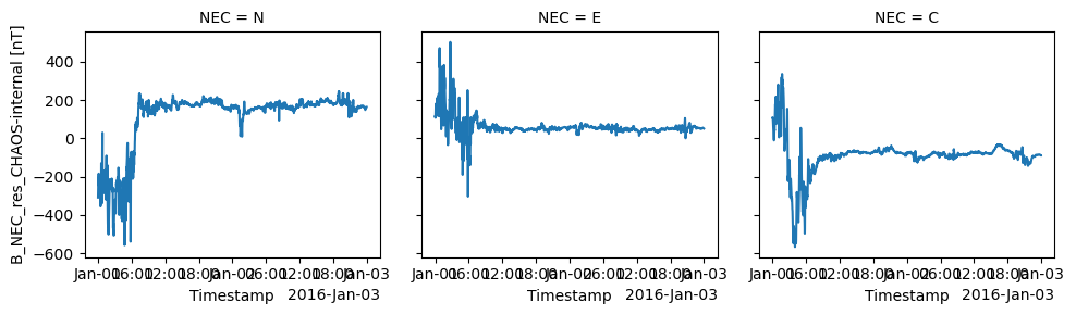
(This roughly shows the disturbance sensed by the observatory due to the magnetospheric and ionospheric sources)

Data visualisation

Three observatories over a year

Let’s run through a visualisation of one year of hourly means from three observatories.

First fetch the data from our chosen observatories across the UK: LER (Lerwick), ESK (Eskdalemuir), HAD (Hartland). We can apply a few optional settings to reduce unnecessary output:

• verbose=False to disable the data terms message

• asynchronous=False to enable synchronous processing on the server - it will be slightly faster but only works for smaller data requests

• show_progress=False to hide the progress bars

request = SwarmRequest()
request.set_collection("SW_OPER_AUX_OBSH2_:LER", verbose=False)
request.set_products(measurements=["B_NEC"])
data = request.get_between("2013-01-01", "2014-01-01", asynchronous=False, show_progress=False)
ds_ler = data.as_xarray()

request = SwarmRequest()
request.set_collection("SW_OPER_AUX_OBSH2_:ESK", verbose=False)
request.set_products(measurements=["B_NEC"])
data = request.get_between("2013-01-01", "2014-01-01", asynchronous=False, show_progress=False)
ds_esk = data.as_xarray()

request = SwarmRequest()
request.set_collection("SW_OPER_AUX_OBSH2_:HAD", verbose=False)
request.set_products(measurements=["B_NEC"])
data = request.get_between("2013-01-01", "2014-01-01", asynchronous=False, show_progress=False)
ds_had = data.as_xarray()

Now our data is in three objects which look like this:

ds_ler

<xarray.Dataset>
Dimensions:    (Timestamp: 8760, NEC: 3)
Coordinates:
  * Timestamp  (Timestamp) datetime64[ns] 2013-01-01T00:30:00 ... 2013-12-31T...
  * NEC        (NEC) <U1 'N' 'E' 'C'
Data variables:
    Longitude  (Timestamp) float64 358.8 358.8 358.8 358.8 ... 358.8 358.8 358.8
    Radius     (Timestamp) float64 6.362e+06 6.362e+06 ... 6.362e+06 6.362e+06
    Latitude   (Timestamp) float64 59.97 59.97 59.97 59.97 ... 59.97 59.97 59.97
    B_NEC      (Timestamp, NEC) float64 1.487e+04 -616.8 ... -561.9 4.862e+04
Attributes:
    Sources:         ['SW_OPER_AUX_OBS_2__20130101T000000_20131231T235959_0141']
    MagneticModels:  []
    AppliedFilters:  []

xarray.Dataset

• Dimensions:
  • Timestamp: 8760
  • NEC: 3
• Coordinates: (2)
  • Timestamp
    (Timestamp)
    datetime64[ns]
    2013-01-01T00:30:00 ... 2013-12-...

    description :

    Date and time

    array(['2013-01-01T00:30:00.000000000', '2013-01-01T01:30:00.000000000',
           '2013-01-01T02:30:00.000000000', ..., '2013-12-31T21:30:00.000000000',
           '2013-12-31T22:30:00.000000000', '2013-12-31T23:30:00.000000000'],
          dtype='datetime64[ns]')

  • NEC
    (NEC)
    <U1
    'N' 'E' 'C'

    units :

    description :

    NEC frame - North, East, Centre (down)

    array(['N', 'E', 'C'], dtype='<U1')

• Data variables: (4)
  • Longitude
    (Timestamp)
    float64
    358.8 358.8 358.8 ... 358.8 358.8

    units :

    deg

    description :

    Longitude

    array([358.817, 358.817, 358.817, ..., 358.817, 358.817, 358.817])

  • Radius
    (Timestamp)
    float64
    6.362e+06 6.362e+06 ... 6.362e+06

    units :

    m

    description :

    Geocentric radius

    array([6362174., 6362174., 6362174., ..., 6362174., 6362174., 6362174.])

  • Latitude
    (Timestamp)
    float64
    59.97 59.97 59.97 ... 59.97 59.97

    units :

    deg

    description :

    Geocentric latitude

    array([59.967, 59.967, 59.967, ..., 59.967, 59.967, 59.967])

  • B_NEC
    (Timestamp, NEC)
    float64
    1.487e+04 -616.8 ... 4.862e+04

    units :

    nT

    description :

    Geocentric-north, east, and geocentric-down component of magnetic field. NaN values are used as placeholders for missing data.

    array([[14865.9,  -616.8, 48595.4],
           [14864.9,  -615.8, 48596.4],
           [14864.9,  -616.8, 48597.4],
           ...,
           [14876.8,  -561.9, 48619.4],
           [14875.8,  -562.9, 48619.4],
           [14876.8,  -561.9, 48617.4]])

• Indexes: (2)
  • Timestamp
    PandasIndex

    PandasIndex(DatetimeIndex(['2013-01-01 00:30:00', '2013-01-01 01:30:00',
                   '2013-01-01 02:30:00', '2013-01-01 03:30:00',
                   '2013-01-01 04:30:00', '2013-01-01 05:30:00',
                   '2013-01-01 06:30:00', '2013-01-01 07:30:00',
                   '2013-01-01 08:30:00', '2013-01-01 09:30:00',
                   ...
                   '2013-12-31 14:30:00', '2013-12-31 15:30:00',
                   '2013-12-31 16:30:00', '2013-12-31 17:30:00',
                   '2013-12-31 18:30:00', '2013-12-31 19:30:00',
                   '2013-12-31 20:30:00', '2013-12-31 21:30:00',
                   '2013-12-31 22:30:00', '2013-12-31 23:30:00'],
                  dtype='datetime64[ns]', name='Timestamp', length=8760, freq=None))

  • NEC
    PandasIndex

    PandasIndex(Index(['N', 'E', 'C'], dtype='object', name='NEC'))

• Attributes: (3)

  Sources :

  ['SW_OPER_AUX_OBS_2__20130101T000000_20131231T235959_0141']

  MagneticModels :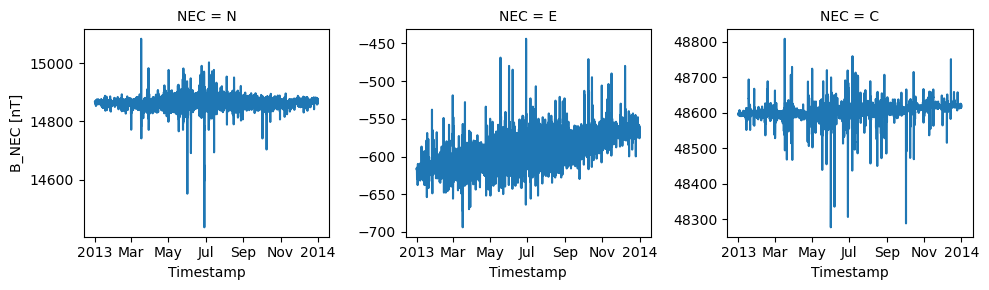

  []

  AppliedFilters :

  []

We can quickly preview the data using the xarray plotting tools:

ds_ler["B_NEC"].plot.line(x="Timestamp", col="NEC", sharey=False)

<xarray.plot.facetgrid.FacetGrid at 0x7fdea7872fd0>

Let’s make a more complex figure to display data from all three observatories together. We can use matplotlib directly now to create the figure and pass the xarray objects to it to fill the contents. Note that we slice out a particular vector component with e.g. ds_ler["B_NEC"].sel(NEC="N").

fig, axes = plt.subplots(nrows=3, ncols=3, figsize=(15, 5), sharex="all", sharey="row")
for i, NEC in enumerate("NEC"):
    axes[i, 0].plot(ds_ler["Timestamp"], ds_ler["B_NEC"].sel(NEC=NEC))
    axes[i, 1].plot(ds_esk["Timestamp"], ds_esk["B_NEC"].sel(NEC=NEC))
    axes[i, 2].plot(ds_had["Timestamp"], ds_had["B_NEC"].sel(NEC=NEC))
    axes[i, 0].set_ylabel(f"B ({NEC}) [nT]")
axes[0, 0].set_title("LER: Lerwick (60.0°N)")
axes[0, 1].set_title("ESK: Eskdalemuir (55.1°N)")
axes[0, 2].set_title("HAD: Hartland (50.8°N)")
fig.tight_layout()

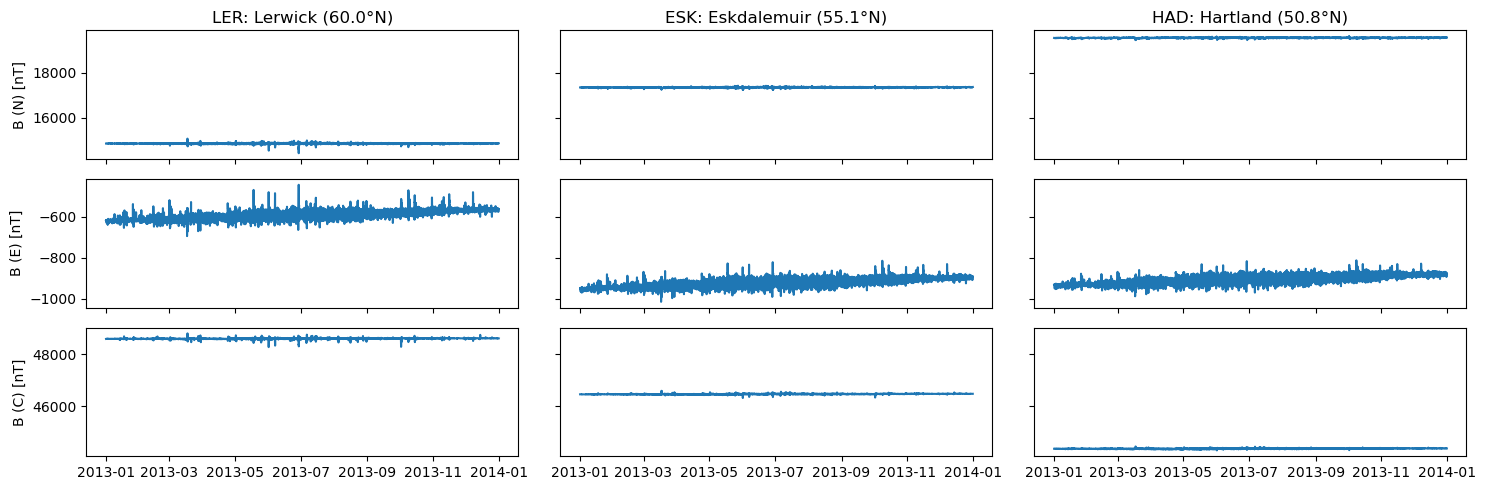
This shows us the difference in the main field between these locations - further North (Lerwick), the field is pointing more downwards so the vertical component (C) is stronger. We can also see a small secular variation over the year as the field changes.