EFIxTIE (Ion temperatures)#
Abstract: Access to the EFIxTIE data product containing estimates of the O+ ion temperature in the upper F region along Swarm orbits.
Documentation:
# Display important package versions used
%load_ext watermark
%watermark -i -v -p viresclient,pandas,xarray,matplotlib
Python implementation: CPython
Python version       : 3.11.6
IPython version      : 8.18.0

viresclient: 0.15.0
pandas     : 2.1.3
xarray     : 2023.12.0
matplotlib : 3.8.2
import datetime as dt

import matplotlib as mpl
import matplotlib.pyplot as plt
import numpy as np
import xarray as xr

# Control the HTML display of the datasets
xr.set_options(
    display_expand_attrs=False, display_expand_coords=True, display_expand_data=True
)

from viresclient import SwarmRequest
request = SwarmRequest()
What data is available?#
There are three collections available, one for each Swarm spacecraft.
request.available_collections("EFI_TIE", details=False)
{'EFI_TIE': ['SW_OPER_EFIATIE_2_', 'SW_OPER_EFIBTIE_2_', 'SW_OPER_EFICTIE_2_']}
print(request.available_measurements("EFI_TIE"))
['Latitude_GD', 'Longitude_GD', 'Height_GD', 'Radius_GC', 'Latitude_QD', 'MLT_QD', 'Tn_msis', 'Te_adj_LP', 'Ti_meas_drift', 'Ti_model_drift', 'Flag_ti_meas', 'Flag_ti_model']
Notes for the listed available variables:
tie_vars = [
    # Positional information in geodetic (GD) and geocentric (GC) frames
    #  redundant with VirES variables Latitude, Longitude, Radius (in geocentric frame)
    "Latitude_GD",
    "Longitude_GD",
    "Height_GD",
    "Radius_GC",
    # Quasi-dipole magnetic latitude and local time
    #  redundant with VirES auxiliaries, QDLat & MLT
    "Latitude_QD",
    "MLT_QD",
    # Neutral temperature from NRLMSISE-00 model
    "Tn_msis",
    # Corrected Swarm LP electron temperature
    "Te_adj_LP",
    # Estimated ion temperature from TII drift at high latitudes
    "Ti_meas_drift",
    # Estimated Ion temperature from Weimer 2005 model drifts at high latitudes
    "Ti_model_drift",
    # Bitwise flags with process information
    #  See the Product definition document for details
    "Flag_ti_meas",
    "Flag_ti_model",
]
Fetching and plotting data#
Hint: you can identify start/end times of specific orbit numbers using .get_times_for_orbits:
request = SwarmRequest()
request.get_times_for_orbits(3740, 3742, mission="Swarm", spacecraft="Alpha")
(datetime.datetime(2014, 7, 25, 1, 9, 37, 149985),
 datetime.datetime(2014, 7, 25, 5, 51, 25, 595024))
For demonstration, we will fetch some data from Swarm Alpha (SW_OPER_EFIATIE_2_). We also ask for magnetic local time, MLT, and orbital information: OrbitNumber, OrbitDirection which can be useful for some plots.
start = dt.datetime(2014, 7, 25, 1, 9, 38)
end = dt.datetime(2014, 7, 25, 5, 51, 25)

request = SwarmRequest()
request.set_collection("SW_OPER_EFIATIE_2_")
request.set_products(
    measurements=tie_vars, auxiliaries=["OrbitNumber", "OrbitDirection", "MLT"]
)
data = request.get_between(start, end)
Data can be loaded as either a pandas datframe or a xarray dataset.
df = data.as_dataframe()
df.head()
| OrbitNumber | Ti_model_drift | Longitude_GD | MLT | Te_adj_LP | Latitude | MLT_QD | Radius | Flag_ti_model | Latitude_GD | Tn_msis | OrbitDirection | Latitude_QD | Longitude | Ti_meas_drift | Radius_GC | Spacecraft | Flag_ti_meas | Height_GD | |
|---|---|---|---|---|---|---|---|---|---|---|---|---|---|---|---|---|---|---|---|
| Timestamp | |||||||||||||||||||
| 2014-07-25 01:09:38.196999936 | 3740 | 1308.57 | -126.081803 | 16.776039 | 1486.15 | -0.012119 | 16.734770 | 6.845324e+06 | 3 | -0.012195 | 1048.83 | 1 | 4.363832 | -126.081803 | 1308.57 | 6.845324e+06 | A | 3 | 467186.573954 |
| 2014-07-25 01:09:38.696000000 | 3740 | 1308.26 | -126.082416 | 16.775776 | 1485.50 | 0.019726 | 16.734495 | 6.845318e+06 | 3 | 0.019850 | 1048.90 | 1 | 4.395916 | -126.082416 | 1308.26 | 6.845318e+06 | A | 3 | 467180.926784 |
| 2014-07-25 01:09:39.196992256 | 3740 | 1308.20 | -126.083031 | 16.775513 | 1484.76 | 0.051698 | 16.734220 | 6.845312e+06 | 3 | 0.052023 | 1048.98 | 1 | 4.428128 | -126.083031 | 1308.20 | 6.845312e+06 | A | 3 | 467175.265855 |
| 2014-07-25 01:09:39.696000000 | 3740 | 1308.21 | -126.083644 | 16.775248 | 1484.88 | 0.083543 | 16.733945 | 6.845307e+06 | 3 | 0.084067 | 1049.05 | 1 | 4.460213 | -126.083644 | 1308.21 | 6.845307e+06 | A | 3 | 467169.641168 |
| 2014-07-25 01:09:40.196999936 | 3740 | 1309.25 | -126.084259 | 16.774982 | 1486.79 | 0.115515 | 16.733669 | 6.845301e+06 | 3 | 0.116240 | 1049.14 | 1 | 4.492427 | -126.084259 | 1309.25 | 6.845301e+06 | A | 3 | 467164.002862 |
ds = data.as_xarray()
ds
<xarray.Dataset>
Dimensions:         (Timestamp: 33808)
Coordinates:
  * Timestamp       (Timestamp) datetime64[ns] 2014-07-25T01:09:38.196999936 ...
Data variables: (12/19)
    Spacecraft      (Timestamp) object 'A' 'A' 'A' 'A' 'A' ... 'A' 'A' 'A' 'A'
    OrbitNumber     (Timestamp) int32 3740 3740 3740 3740 ... 3742 3742 3742
    Ti_model_drift  (Timestamp) float64 1.309e+03 1.308e+03 ... 1.279e+03
    Longitude_GD    (Timestamp) float64 -126.1 -126.1 -126.1 ... 163.2 163.2
    MLT             (Timestamp) float64 16.78 16.78 16.78 ... 16.6 16.6 16.6
    Te_adj_LP       (Timestamp) float64 1.486e+03 1.486e+03 ... 1.98e+03
    ...              ...
    Latitude_QD     (Timestamp) float64 4.364 4.396 4.428 ... -6.095 -6.063
    Longitude       (Timestamp) float64 -126.1 -126.1 -126.1 ... 163.2 163.2
    Ti_meas_drift   (Timestamp) float64 1.309e+03 1.308e+03 ... 1.279e+03
    Radius_GC       (Timestamp) float64 6.845e+06 6.845e+06 ... 6.845e+06
    Flag_ti_meas    (Timestamp) uint8 3 3 3 3 3 3 3 3 3 3 ... 1 1 1 1 1 1 1 1 1
    Height_GD       (Timestamp) float64 4.672e+05 4.672e+05 ... 4.673e+05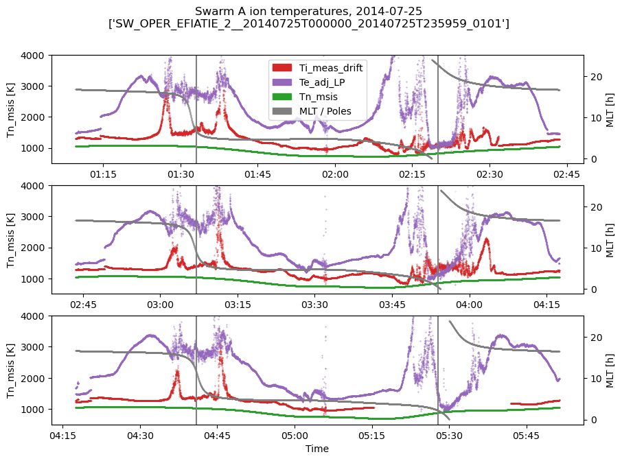
Attributes: (3)# Set up a time series plot where each row is an orbit
nrows = len(np.unique(ds["OrbitNumber"]))
fig, axes = plt.subplots(nrows=nrows, ncols=1, figsize=(10, 7))
axes_r = [ax.twinx() for ax in axes]
for i, (orbitnumber, ds_orbit) in enumerate(ds.groupby("OrbitNumber")):
# Plot electron & ion temperatures, measured and modelled
ds_orbit.plot.scatter(
x="Timestamp", y="Ti_meas_drift", s=0.1, ax=axes[i], color="tab:red"
)
ds_orbit.plot.scatter(
x="Timestamp", y="Te_adj_LP", s=0.1, ax=axes[i], color="tab:purple"
)
ds_orbit.plot.scatter(
x="Timestamp", y="Tn_msis", s=0.1, ax=axes[i], color="tab:green"
)
ds_orbit.plot.scatter(
x="Timestamp", y="MLT", s=0.05, ax=axes_r[i], color="tab:gray", alpha=0.5
)
# Identify times closest to North and South pole
t_NP = ds_orbit["Timestamp"].isel(Timestamp=ds_orbit["Latitude"].argmax()).values
t_SP = ds_orbit["Timestamp"].isel(Timestamp=ds_orbit["Latitude"].argmin()).values
axes[i].axvline(mpl.dates.date2num(t_NP), color="gray")
axes[i].axvline(mpl.dates.date2num(t_SP), color="gray")
# Tidy up labelling
axes[i].xaxis.set_major_formatter(mpl.dates.DateFormatter("%H:%M"))
axes[i].set_xlabel("")
# Add legend manually
red = mpl.patches.Patch(color="tab:red", label="Ti_meas_drift")
purple = mpl.patches.Patch(color="tab:purple", label="Te_adj_LP")
green = mpl.patches.Patch(color="tab:green", label="Tn_msis")
gray = mpl.patches.Patch(color="tab:gray", label="MLT / Poles")
axes[0].legend(handles=[red, purple, green, gray])
# Tidy up axes and labelling
for ax in axes:
ax.set_ylim(500, 4000)
axes[-1].set_xlabel("Time")
title = "".join(
[
f"Swarm {ds['Spacecraft'].data[0]} ion temperatures, ",
ds["Timestamp"].dt.date.data[0].isoformat(),
f"\n{[s for s in ds.attrs['Sources'] if 'TIE' in s]}",
]
)
fig.suptitle(title);