Geomagnetic Model Residuals

Abstract: An exploration of geomagnetic data-model residuals evaluated through VirES (along Swarm orbits).

%load_ext watermark
%watermark -i -v -p viresclient,pandas,xarray,matplotlib

Python implementation: CPython
Python version       : 3.11.6
IPython version      : 8.18.0

viresclient: 0.11.6
pandas     : 2.1.3
xarray     : 2023.12.0
matplotlib : 3.8.2

from viresclient import SwarmRequest
import matplotlib.pyplot as plt

One day of residuals

(data minus a core field model)

request = SwarmRequest()
request.set_collection("SW_OPER_MAGA_LR_1B")
request.set_products(
    measurements=["B_NEC"],
    models=["CHAOS-Core"],
    residuals=True,
    sampling_step="PT5S",
    auxiliaries=["MLT", "QDLat", "SunZenithAngle"]
)
data = request.get_between(
    "2019-01-01", "2019-01-02",
    asynchronous=False, show_progress=False
)
ds = data.as_xarray()
ds

<xarray.Dataset>
Dimensions:               (Timestamp: 17280, NEC: 3)
Coordinates:
  * Timestamp             (Timestamp) datetime64[ns] 2019-01-01 ... 2019-01-0...
  * NEC                   (NEC) <U1 'N' 'E' 'C'
Data variables:
    Spacecraft            (Timestamp) object 'A' 'A' 'A' 'A' ... 'A' 'A' 'A' 'A'
    MLT                   (Timestamp) float64 14.8 14.79 14.79 ... 2.419 2.419
    B_NEC_res_CHAOS-Core  (Timestamp, NEC) float64 -12.93 -19.23 ... 5.861 7.215
    Radius                (Timestamp) float64 6.819e+06 6.819e+06 ... 6.809e+06
    Latitude              (Timestamp) float64 -17.03 -16.71 ... 44.51 44.19
    SunZenithAngle        (Timestamp) float64 40.87 40.97 41.08 ... 141.0 141.1
    QDLat                 (Timestamp) float64 -13.95 -13.63 ... 40.36 40.02
    Longitude             (Timestamp) float64 -136.0 -136.0 ... 40.87 40.88
Attributes:
    Sources:         ['SW_OPER_MCO_SHA_2X_19970101T000000_20240207T235959_071...
    MagneticModels:  ["CHAOS-Core = 'CHAOS-Core'(max_degree=20,min_degree=1)"]
    AppliedFilters:  []

xarray.Dataset

• Dimensions:
  • Timestamp: 17280
  • NEC: 3
• Coordinates: (2)
  • Timestamp
    (Timestamp)
    datetime64[ns]
    2019-01-01 ... 2019-01-01T23:59:55

    description :

    Time stamp

    array(['2019-01-01T00:00:00.000000000', '2019-01-01T00:00:05.000000000',
           '2019-01-01T00:00:10.000000000', ..., '2019-01-01T23:59:45.000000000',
           '2019-01-01T23:59:50.000000000', '2019-01-01T23:59:55.000000000'],
          dtype='datetime64[ns]')

  • NEC
    (NEC)
    <U1
    'N' 'E' 'C'

    units :

    description :

    NEC frame - North, East, Centre (down)

    array(['N', 'E', 'C'], dtype='<U1')

• Data variables: (8)
  • Spacecraft
    (Timestamp)
    object
    'A' 'A' 'A' 'A' ... 'A' 'A' 'A' 'A'

    units :

    -

    description :

    Spacecraft identifier (values: 'A', 'B', 'C' or '-' if not available).

    array(['A', 'A', 'A', ..., 'A', 'A', 'A'], dtype=object)

  • MLT
    (Timestamp)
    float64
    14.8 14.79 14.79 ... 2.419 2.419

    units :

    h

    description :

    Magnetic local time

    array([14.79740524, 14.79370308, 14.79004192, ...,  2.41829491,
            2.41878891,  2.41931725])

  • B_NEC_res_CHAOS-Core
    (Timestamp, NEC)
    float64
    -12.93 -19.23 ... 5.861 7.215

    units :

    nT

    description :

    Magnetic field vector residual, NEC frame, calculated as a difference of the measurement and value of the CHAOS-Core spherical harmonic model

    array([[-12.93328926, -19.22730367,  -1.29154661],
           [-13.02661147, -20.1710537 ,  -2.09730326],
           [-12.4973703 , -22.17165392,  -2.23270223],
           ...,
           [-15.20469534,   5.50923518,   6.5459321 ],
           [-15.81153038,   5.73691094,   6.78088348],
           [-16.45115364,   5.86102995,   7.2150089 ]])

  • Radius
    (Timestamp)
    float64
    6.819e+06 6.819e+06 ... 6.809e+06

    units :

    m

    description :

    Position in ITRF - Radius

    array([6819106.91, 6819066.61, 6819026.06, ..., 6809057.26, 6809113.39,
           6809169.72])

  • Latitude
    (Timestamp)
    float64
    -17.03 -16.71 ... 44.51 44.19

    units :

    deg

    description :

    Position in ITRF - Latitude

    array([-17.0299019, -16.7090917, -16.388275 , ...,  44.8308038,
            44.5095444,  44.1882802])

  • SunZenithAngle
    (Timestamp)
    float64
    40.87 40.97 41.08 ... 141.0 141.1

    units :

    deg

    description :

    Sun position - zenith angle

    array([ 40.86874699,  40.97170449,  41.07651982, ..., 140.90588459,
           140.99807308, 141.08820725])

  • QDLat
    (Timestamp)
    float64
    -13.95 -13.63 ... 40.36 40.02

    units :

    deg

    description :

    Magnetic quasi-dipole latitude

    array([-13.95402908, -13.63445377, -13.31469536, ...,  40.70093918,
            40.36060333,  40.02004623])

  • Longitude
    (Timestamp)
    float64
    -136.0 -136.0 ... 40.87 40.88

    units :

    deg

    description :

    Position in ITRF - Longitude

    array([-136.0207597, -136.0254153, -136.0301253, ...,   40.8610347,
             40.8696294,   40.8779002])

• Indexes: (2)
  • Timestamp
    PandasIndex

    PandasIndex(DatetimeIndex(['2019-01-01 00:00:00', '2019-01-01 00:00:05',
                   '2019-01-01 00:00:10', '2019-01-01 00:00:15',
                   '2019-01-01 00:00:20', '2019-01-01 00:00:25',
                   '2019-01-01 00:00:30', '2019-01-01 00:00:35',
                   '2019-01-01 00:00:40', '2019-01-01 00:00:45',
                   ...
                   '2019-01-01 23:59:10', '2019-01-01 23:59:15',
                   '2019-01-01 23:59:20', '2019-01-01 23:59:25',
                   '2019-01-01 23:59:30', '2019-01-01 23:59:35',
                   '2019-01-01 23:59:40', '2019-01-01 23:59:45',
                   '2019-01-01 23:59:50', '2019-01-01 23:59:55'],
                  dtype='datetime64[ns]', name='Timestamp', length=17280, freq=None))

  • NEC
    PandasIndex

    PandasIndex(Index(['N', 'E', 'C'], dtype='object', name='NEC'))

• Attributes: (3)

  Sources :

  ['SW_OPER_MCO_SHA_2X_19970101T000000_20240207T235959_0716', 'SW_PREL_MAGA_LR_1B_20190101T000000_20190101T235959_0603_MDR_MAG_LR']

  MagneticModels :

  ["CHAOS-Core = 'CHAOS-Core'(max_degree=20,min_degree=1)"]

  AppliedFilters :

  []

xarray provides some convenient direct plotting tools through integration with matplotlib:

ds["B_NEC_res_CHAOS-Core"].plot.line(x="Timestamp");

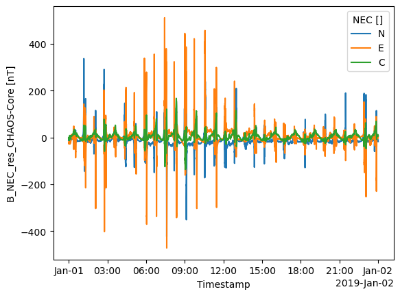
This allows some very compact plotting commands to create complex figures, if you know how! This kind of plotting takes a while to learn and experiment with to get right, but results in short and manageable code.

facetgrid = ds.plot.scatter(x="QDLat", y="B_NEC_res_CHAOS-Core", col="NEC",
                s=1, hue="SunZenithAngle", cmap="hot_r", alpha=0.6, linewidths=0)
for ax in facetgrid.axs.flat:
    ax.set_facecolor("grey")

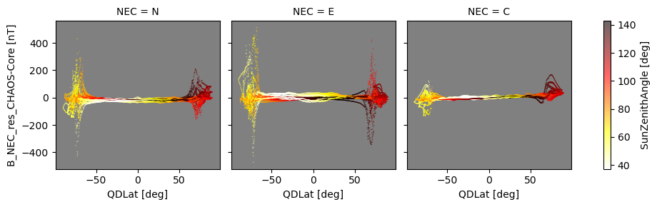
(showing that we are in daylight more in the Southern hemisphere, while in darkness in the Northern, because the data is from January - Northern winter)

facetgrid = ds.plot.scatter(x="QDLat", y="B_NEC_res_CHAOS-Core", col="NEC",
                s=1, hue="MLT", cmap="twilight_shifted", alpha=0.6, linewidths=0)
for ax in facetgrid.axs.flat:
    ax.set_facecolor("grey")

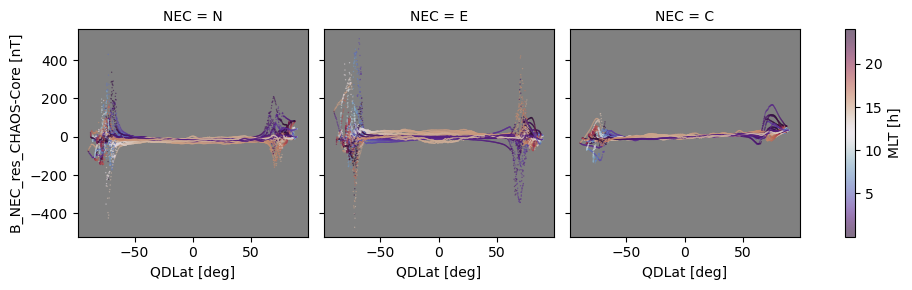
(showing the rapid movement through local time sectors (MLT) when the satellite passes through polar regions)

The above figures show large residuals in the polar regions due to currents in the auroral oval. These cause greater disturbance in the Northward (N) and Eastward (E) components of the magnetic field because of the geometry of the field-aligned currents (FACs) which cause the magnetic disturbance.

Access 1 year of data and models

Let’s inspect a whole year of data (at 2-minute sampling):

• The B_NEC vector from Swarm Alpha

• All parts of the CHAOS model (core, crust, magnetosphere) evaluated at the same points

• MLT, QDLat, and SunZenithAngle which are also evaluated on-the-fly

• Filtered to remove some bad data (according to Flags_F) and restricted to geomagnetically quiet data (according to Kp)

We fetch the model values themselves as well as the measurements (instead of just the residuals as above) so that we can manipulate all the different components locally.

Warning: This will take several minutes to process

request = SwarmRequest()
request.set_collection("SW_OPER_MAGA_LR_1B")
request.set_products(
    measurements=["B_NEC"],
    models=["CHAOS-Core", "CHAOS-Static", "CHAOS-MMA-Primary", "CHAOS-MMA-Secondary"],
    auxiliaries=["MLT", "QDLat", "SunZenithAngle", "OrbitNumber"],
    sampling_step="PT120S"
)
request.set_range_filter("Flags_F", 0, 1)
request.set_range_filter("Kp", 0, 3)
# request.set_range_filter("SunZenithAngle", 100, 180)
data = request.get_between("2019-01-01", "2020-01-01")
ds = data.as_xarray()
# Remove the extra-long Sources list
ds.attrs["Sources"] = "Many"
ds

<xarray.Dataset>
Dimensions:                    (Timestamp: 242598, NEC: 3)
Coordinates:
  * Timestamp                  (Timestamp) datetime64[ns] 2019-01-01 ... 2019...
  * NEC                        (NEC) <U1 'N' 'E' 'C'
Data variables: (12/13)
    Spacecraft                 (Timestamp) object 'A' 'A' 'A' ... 'A' 'A' 'A'
    MLT                        (Timestamp) float64 14.8 14.72 ... 6.219 6.348
    B_NEC_CHAOS-Static         (Timestamp, NEC) float64 -0.1243 1.575 ... 0.5559
    B_NEC_CHAOS-Core           (Timestamp, NEC) float64 2.369e+04 ... 4.915e+04
    B_NEC                      (Timestamp, NEC) float64 2.368e+04 ... 4.915e+04
    OrbitNumber                (Timestamp) int32 28692 28692 ... 34324 34324
    ...                         ...
    Latitude                   (Timestamp) float64 -17.03 -9.329 ... 61.38 69.06
    B_NEC_CHAOS-MMA-Secondary  (Timestamp, NEC) float64 -0.303 0.9856 ... 1.384
    B_NEC_CHAOS-MMA-Primary    (Timestamp, NEC) float64 -13.85 1.0 ... 5.657
    SunZenithAngle             (Timestamp) float64 40.87 43.82 ... 107.4 108.7
    QDLat                      (Timestamp) float64 -13.95 -6.242 ... 57.39 64.82
    Longitude                  (Timestamp) float64 -136.0 -136.1 ... 97.65 99.22
Attributes:
    Sources:         Many
    MagneticModels:  ["CHAOS-Core = 'CHAOS-Core'(max_degree=20,min_degree=1)"...
    AppliedFilters:  ['Flags_F <= 1', 'Flags_F >= 0', 'Kp <= 3', 'Kp >= 0']

xarray.Dataset

• Dimensions:
  • Timestamp: 242598
  • NEC: 3
• Coordinates: (2)
  • Timestamp
    (Timestamp)
    datetime64[ns]
    2019-01-01 ... 2019-12-31T23:58:00

    description :

    Time stamp

    array(['2019-01-01T00:00:00.000000000', '2019-01-01T00:02:00.000000000',
           '2019-01-01T00:04:00.000000000', ..., '2019-12-31T23:54:00.000000000',
           '2019-12-31T23:56:00.000000000', '2019-12-31T23:58:00.000000000'],
          dtype='datetime64[ns]')

  • NEC
    (NEC)
    <U1
    'N' 'E' 'C'

    units :

    description :

    NEC frame - North, East, Centre (down)

    array(['N', 'E', 'C'], dtype='<U1')

• Data variables: (13)
  • Spacecraft
    (Timestamp)
    object
    'A' 'A' 'A' 'A' ... 'A' 'A' 'A' 'A'

    units :

    -

    description :

    Spacecraft identifier (values: 'A', 'B', 'C' or '-' if not available).

    array(['A', 'A', 'A', ..., 'A', 'A', 'A'], dtype=object)

  • MLT
    (Timestamp)
    float64
    14.8 14.72 14.65 ... 6.219 6.348

    units :

    h

    description :

    Magnetic local time

    array([14.79740524, 14.71789551, 14.65094757, ...,  6.12784386,
            6.21863174,  6.34835625])

  • B_NEC_CHAOS-Static
    (Timestamp, NEC)
    float64
    -0.1243 1.575 ... 2.338 0.5559

    units :

    nT

    description :

    Magnetic field vector, NEC frame, calculated by the CHAOS-Static spherical harmonic model

    array([[-0.12427424,  1.57504536, -0.36996116],
           [ 0.06280141,  0.72170757, -0.4087065 ],
           [ 0.17748272, -0.388705  ,  0.30508599],
           ...,
           [-0.47221455, -0.03294338, -0.95104102],
           [ 0.83005169, -1.69760825,  1.27594809],
           [ 1.93739102,  2.33844637,  0.55589511]])

  • B_NEC_CHAOS-Core
    (Timestamp, NEC)
    float64
    2.369e+04 5.314e+03 ... 4.915e+04

    units :

    nT

    description :

    Magnetic field vector, NEC frame, calculated by the CHAOS-Core spherical harmonic model

    array([[ 2.36889341e+04,  5.31437820e+03, -1.22471230e+04],
           [ 2.45843273e+04,  4.72325850e+03, -5.58645030e+03],
           [ 2.48485956e+04,  4.28227312e+03,  1.28326544e+03],
           ...,
           [ 1.40755929e+04, -4.19168816e+01,  4.66759050e+04],
           [ 9.73758897e+03,  1.20689105e+02,  4.86426646e+04],
           [ 6.01301505e+03,  2.72187878e+02,  4.91454266e+04]])

  • B_NEC
    (Timestamp, NEC)
    float64
    2.368e+04 5.295e+03 ... 4.915e+04

    units :

    nT

    description :

    Magnetic field vector, NEC frame

    array([[ 2.36760008e+04,  5.29515090e+03, -1.22484145e+04],
           [ 2.45740495e+04,  4.69856949e+03, -5.59765010e+03],
           [ 2.48499011e+04,  4.26006984e+03,  1.28627100e+03],
           ...,
           [ 1.40708616e+04, -4.05193482e+01,  4.66819932e+04],
           [ 9.73489373e+03,  1.19725402e+02,  4.86510680e+04],
           [ 6.01312094e+03,  2.77310333e+02,  4.91516582e+04]])

  • OrbitNumber
    (Timestamp)
    int32
    28692 28692 28692 ... 34324 34324

    units :

    -

    description :

    Orbit number (set to -1 if not available)

    array([28692, 28692, 28692, ..., 34324, 34324, 34324], dtype=int32)

  • Radius
    (Timestamp)
    float64
    6.819e+06 6.818e+06 ... 6.803e+06

    units :

    m

    description :

    Position in ITRF - Radius

    array([6819106.91, 6818073.77, 6816909.52, ..., 6805320.65, 6804302.47,
           6803498.32])

  • Latitude
    (Timestamp)
    float64
    -17.03 -9.329 ... 61.38 69.06

    units :

    deg

    description :

    Position in ITRF - Latitude

    array([-17.0299019,  -9.3287281,  -1.6242172, ...,  53.6733283,
            61.3772633,  69.0629806])

  • B_NEC_CHAOS-MMA-Secondary
    (Timestamp, NEC)
    float64
    -0.303 0.9856 ... -1.142 1.384

    units :

    nT

    description :

    Magnetic field vector, NEC frame, calculated by the CHAOS-MMA-Secondary spherical harmonic model

    array([[-0.30297056,  0.98564803, -2.89135236],
           [-0.10470823,  0.87585609, -2.91108254],
           [ 0.08722358,  0.76643363, -2.88592763],
           ...,
           [ 0.32726343, -1.21991201,  1.31986096],
           [ 0.16572226, -1.17265426,  1.38592177],
           [ 0.01670538, -1.14231647,  1.38397679]])

  • B_NEC_CHAOS-MMA-Primary
    (Timestamp, NEC)
    float64
    -13.85 1.0 1.269 ... -3.015 5.657

    units :

    nT

    description :

    Magnetic field vector, NEC frame, calculated by the CHAOS-MMA-Primary spherical harmonic model

    array([[-13.85326293,   1.00041826,   1.26932794],
           [-13.57361511,   0.72772099,   2.95157387],
           [-13.10998322,   0.45323748,   4.58952267],
           ...,
           [ -5.35689486,  -3.26147668,   4.64691082],
           [ -4.63973588,  -3.10838554,   5.19147355],
           [ -3.83557873,  -3.01480717,   5.65749524]])

  • SunZenithAngle
    (Timestamp)
    float64
    40.87 43.82 47.65 ... 107.4 108.7

    units :

    deg

    description :

    Sun position - zenith angle

    array([ 40.86874699,  43.82230911,  47.64623674, ..., 105.76064586,
           107.38050934, 108.68561163])

  • QDLat
    (Timestamp)
    float64
    -13.95 -6.242 1.515 ... 57.39 64.82

    units :

    deg

    description :

    Magnetic quasi-dipole latitude

    array([-13.95402908,  -6.24187136,   1.51521564, ...,  49.68329239,
            57.39051437,  64.82193756])

  • Longitude
    (Timestamp)
    float64
    -136.0 -136.1 ... 97.65 99.22

    units :

    deg

    description :

    Position in ITRF - Longitude

    array([-136.0207597, -136.1450285, -136.2855785, ...,   96.8970934,
             97.6468168,   99.2203183])

• Indexes: (2)
  • Timestamp
    PandasIndex

    PandasIndex(DatetimeIndex(['2019-01-01 00:00:00', '2019-01-01 00:02:00',
                   '2019-01-01 00:04:00', '2019-01-01 00:06:00',
                   '2019-01-01 00:08:00', '2019-01-01 00:10:00',
                   '2019-01-01 00:12:00', '2019-01-01 00:14:00',
                   '2019-01-01 00:16:00', '2019-01-01 00:18:00',
                   ...
                   '2019-12-31 23:40:00', '2019-12-31 23:42:00',
                   '2019-12-31 23:44:00', '2019-12-31 23:46:00',
                   '2019-12-31 23:48:00', '2019-12-31 23:50:00',
                   '2019-12-31 23:52:00', '2019-12-31 23:54:00',
                   '2019-12-31 23:56:00', '2019-12-31 23:58:00'],
                  dtype='datetime64[ns]', name='Timestamp', length=242598, freq=None))

  • NEC
    PandasIndex

    PandasIndex(Index(['N', 'E', 'C'], dtype='object', name='NEC'))

• Attributes: (3)

  Sources :

  Many

  MagneticModels :

  ["CHAOS-Core = 'CHAOS-Core'(max_degree=20,min_degree=1)", "CHAOS-MMA-Primary = 'CHAOS-MMA-Primary'(max_degree=2,min_degree=1)", "CHAOS-MMA-Secondary = 'CHAOS-MMA-Secondary'(max_degree=2,min_degree=1)", "CHAOS-Static = 'CHAOS-Static'(max_degree=185,min_degree=21)"]

  AppliedFilters :

  ['Flags_F <= 1', 'Flags_F >= 0', 'Kp <= 3', 'Kp >= 0']

We can construct xarray.DataArray’s based on ds:

ds["B_NEC"]

<xarray.DataArray 'B_NEC' (Timestamp: 242598, NEC: 3)>
array([[ 2.36760008e+04,  5.29515090e+03, -1.22484145e+04],
       [ 2.45740495e+04,  4.69856949e+03, -5.59765010e+03],
       [ 2.48499011e+04,  4.26006984e+03,  1.28627100e+03],
       ...,
       [ 1.40708616e+04, -4.05193482e+01,  4.66819932e+04],
       [ 9.73489373e+03,  1.19725402e+02,  4.86510680e+04],
       [ 6.01312094e+03,  2.77310333e+02,  4.91516582e+04]])
Coordinates:
  * Timestamp  (Timestamp) datetime64[ns] 2019-01-01 ... 2019-12-31T23:58:00
  * NEC        (NEC) <U1 'N' 'E' 'C'
Attributes:
    units:        nT
    description:  Magnetic field vector, NEC frame

xarray.DataArray

'B_NEC'

• Timestamp: 242598
• NEC: 3

• 2.368e+04 5.295e+03 -1.225e+04 2.457e+04 ... 6.013e+03 277.3 4.915e+04

  array([[ 2.36760008e+04,  5.29515090e+03, -1.22484145e+04],
         [ 2.45740495e+04,  4.69856949e+03, -5.59765010e+03],
         [ 2.48499011e+04,  4.26006984e+03,  1.28627100e+03],
         ...,
         [ 1.40708616e+04, -4.05193482e+01,  4.66819932e+04],
         [ 9.73489373e+03,  1.19725402e+02,  4.86510680e+04],
         [ 6.01312094e+03,  2.77310333e+02,  4.91516582e+04]])

• Coordinates: (2)
  • Timestamp
    (Timestamp)
    datetime64[ns]
    2019-01-01 ... 2019-12-31T23:58:00

    description :

    Time stamp

    array(['2019-01-01T00:00:00.000000000', '2019-01-01T00:02:00.000000000',
           '2019-01-01T00:04:00.000000000', ..., '2019-12-31T23:54:00.000000000',
           '2019-12-31T23:56:00.000000000', '2019-12-31T23:58:00.000000000'],
          dtype='datetime64[ns]')

  • NEC
    (NEC)
    <U1
    'N' 'E' 'C'

    units :

    description :

    NEC frame - North, East, Centre (down)

    array(['N', 'E', 'C'], dtype='<U1')

• Indexes: (2)
  • Timestamp
    PandasIndex

    PandasIndex(DatetimeIndex(['2019-01-01 00:00:00', '2019-01-01 00:02:00',
                   '2019-01-01 00:04:00', '2019-01-01 00:06:00',
                   '2019-01-01 00:08:00', '2019-01-01 00:10:00',
                   '2019-01-01 00:12:00', '2019-01-01 00:14:00',
                   '2019-01-01 00:16:00', '2019-01-01 00:18:00',
                   ...
                   '2019-12-31 23:40:00', '2019-12-31 23:42:00',
                   '2019-12-31 23:44:00', '2019-12-31 23:46:00',
                   '2019-12-31 23:48:00', '2019-12-31 23:50:00',
                   '2019-12-31 23:52:00', '2019-12-31 23:54:00',
                   '2019-12-31 23:56:00', '2019-12-31 23:58:00'],
                  dtype='datetime64[ns]', name='Timestamp', length=242598, freq=None))

  • NEC
    PandasIndex

    PandasIndex(Index(['N', 'E', 'C'], dtype='object', name='NEC'))

• Attributes: (2)

  units :

  nT

  description :

  Magnetic field vector, NEC frame

ds["B_NEC"] - ds["B_NEC_CHAOS-Core"]

<xarray.DataArray (Timestamp: 242598, NEC: 3)>
array([[-12.93328926, -19.22730367,  -1.29154661],
       [-10.27773072, -24.68900976, -11.19980436],
       [  1.30550781, -22.2032852 ,   3.00556135],
       ...,
       [ -4.73135199,   1.39753336,   6.08821302],
       [ -2.69523391,  -0.96370267,   8.40348281],
       [  0.10588504,   5.12245525,   6.23164093]])
Coordinates:
  * Timestamp  (Timestamp) datetime64[ns] 2019-01-01 ... 2019-12-31T23:58:00
  * NEC        (NEC) <U1 'N' 'E' 'C'

xarray.DataArray

• Timestamp: 242598
• NEC: 3

• -12.93 -19.23 -1.292 -10.28 -24.69 ... 8.403 0.1059 5.122 6.232

  array([[-12.93328926, -19.22730367,  -1.29154661],
         [-10.27773072, -24.68900976, -11.19980436],
         [  1.30550781, -22.2032852 ,   3.00556135],
         ...,
         [ -4.73135199,   1.39753336,   6.08821302],
         [ -2.69523391,  -0.96370267,   8.40348281],
         [  0.10588504,   5.12245525,   6.23164093]])

• Coordinates: (2)
  • Timestamp
    (Timestamp)
    datetime64[ns]
    2019-01-01 ... 2019-12-31T23:58:00

    description :

    Time stamp

    array(['2019-01-01T00:00:00.000000000', '2019-01-01T00:02:00.000000000',
           '2019-01-01T00:04:00.000000000', ..., '2019-12-31T23:54:00.000000000',
           '2019-12-31T23:56:00.000000000', '2019-12-31T23:58:00.000000000'],
          dtype='datetime64[ns]')

  • NEC
    (NEC)
    <U1
    'N' 'E' 'C'

    units :

    description :

    NEC frame - North, East, Centre (down)

    array(['N', 'E', 'C'], dtype='<U1')

• Indexes: (2)
  • Timestamp
    PandasIndex

    PandasIndex(DatetimeIndex(['2019-01-01 00:00:00', '2019-01-01 00:02:00',
                   '2019-01-01 00:04:00', '2019-01-01 00:06:00',
                   '2019-01-01 00:08:00', '2019-01-01 00:10:00',
                   '2019-01-01 00:12:00', '2019-01-01 00:14:00',
                   '2019-01-01 00:16:00', '2019-01-01 00:18:00',
                   ...
                   '2019-12-31 23:40:00', '2019-12-31 23:42:00',
                   '2019-12-31 23:44:00', '2019-12-31 23:46:00',
                   '2019-12-31 23:48:00', '2019-12-31 23:50:00',
                   '2019-12-31 23:52:00', '2019-12-31 23:54:00',
                   '2019-12-31 23:56:00', '2019-12-31 23:58:00'],
                  dtype='datetime64[ns]', name='Timestamp', length=242598, freq=None))

  • NEC
    PandasIndex

    PandasIndex(Index(['N', 'E', 'C'], dtype='object', name='NEC'))

• Attributes: (0)

… and we can plot these directly:

(ds["B_NEC"] - ds["B_NEC_CHAOS-Core"]).plot.line(x="Timestamp");

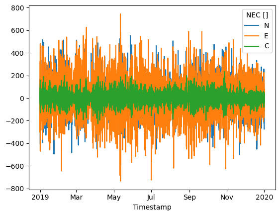
We can slice out a particular time window:

# Selects two days
ds.sel({"Timestamp": slice("2019-01-01", "2019-01-02")})

<xarray.Dataset>
Dimensions:                    (Timestamp: 1415, NEC: 3)
Coordinates:
  * Timestamp                  (Timestamp) datetime64[ns] 2019-01-01 ... 2019...
  * NEC                        (NEC) <U1 'N' 'E' 'C'
Data variables: (12/13)
    Spacecraft                 (Timestamp) object 'A' 'A' 'A' ... 'A' 'A' 'A'
    MLT                        (Timestamp) float64 14.8 14.72 ... 18.85 17.34
    B_NEC_CHAOS-Static         (Timestamp, NEC) float64 -0.1243 ... -0.1479
    B_NEC_CHAOS-Core           (Timestamp, NEC) float64 2.369e+04 ... -4.555e+04
    B_NEC                      (Timestamp, NEC) float64 2.368e+04 ... -4.556e+04
    OrbitNumber                (Timestamp) int32 28692 28692 ... 28723 28723
    ...                         ...
    Latitude                   (Timestamp) float64 -17.03 -9.329 ... -78.6
    B_NEC_CHAOS-MMA-Secondary  (Timestamp, NEC) float64 -0.303 ... 0.03659
    B_NEC_CHAOS-MMA-Primary    (Timestamp, NEC) float64 -13.85 1.0 ... -12.97
    SunZenithAngle             (Timestamp) float64 40.87 43.82 ... 62.83 57.18
    QDLat                      (Timestamp) float64 -13.95 -6.242 ... -72.04
    Longitude                  (Timestamp) float64 -136.0 -136.1 ... -150.7
Attributes:
    Sources:         Many
    MagneticModels:  ["CHAOS-Core = 'CHAOS-Core'(max_degree=20,min_degree=1)"...
    AppliedFilters:  ['Flags_F <= 1', 'Flags_F >= 0', 'Kp <= 3', 'Kp >= 0']

xarray.Dataset

• Dimensions:
  • Timestamp: 1415
  • NEC: 3
• Coordinates: (2)
  • Timestamp
    (Timestamp)
    datetime64[ns]
    2019-01-01 ... 2019-01-02T23:58:00

    description :

    Time stamp

    array(['2019-01-01T00:00:00.000000000', '2019-01-01T00:02:00.000000000',
           '2019-01-01T00:04:00.000000000', ..., '2019-01-02T23:54:00.000000000',
           '2019-01-02T23:56:00.000000000', '2019-01-02T23:58:00.000000000'],
          dtype='datetime64[ns]')

  • NEC
    (NEC)
    <U1
    'N' 'E' 'C'

    units :

    description :

    NEC frame - North, East, Centre (down)

    array(['N', 'E', 'C'], dtype='<U1')

• Data variables: (13)
  • Spacecraft
    (Timestamp)
    object
    'A' 'A' 'A' 'A' ... 'A' 'A' 'A' 'A'

    units :

    -

    description :

    Spacecraft identifier (values: 'A', 'B', 'C' or '-' if not available).

    array(['A', 'A', 'A', ..., 'A', 'A', 'A'], dtype=object)

  • MLT
    (Timestamp)
    float64
    14.8 14.72 14.65 ... 18.85 17.34

    units :

    h

    description :

    Magnetic local time

    array([14.79740524, 14.71789551, 14.65094757, ..., 21.02399826,
           18.85276031, 17.33812141])

  • B_NEC_CHAOS-Static
    (Timestamp, NEC)
    float64
    -0.1243 1.575 ... -1.055 -0.1479

    units :

    nT

    description :

    Magnetic field vector, NEC frame, calculated by the CHAOS-Static spherical harmonic model

    array([[-0.12427424,  1.57504536, -0.36996116],
           [ 0.06280141,  0.72170757, -0.4087065 ],
           [ 0.17748272, -0.388705  ,  0.30508599],
           ...,
           [ 1.14016156, -2.48500595, -1.8869712 ],
           [ 0.08572008,  1.26166   ,  1.48343422],
           [-1.11922306, -1.05490184, -0.14792811]])

  • B_NEC_CHAOS-Core
    (Timestamp, NEC)
    float64
    2.369e+04 5.314e+03 ... -4.555e+04

    units :

    nT

    description :

    Magnetic field vector, NEC frame, calculated by the CHAOS-Core spherical harmonic model

    array([[ 23688.93412096,   5314.37820454, -12247.12299503],
           [ 24584.32727405,   4723.25850425,  -5586.45029504],
           [ 24848.59563346,   4282.27312359,   1283.26543975],
           ...,
           [ -2223.87979637, -12174.40121416, -42432.16388108],
           [ -7915.49368024,   8001.27686894, -44657.06148192],
           [   -77.15045795,  10922.29262921, -45546.7870622 ]])

  • B_NEC
    (Timestamp, NEC)
    float64
    2.368e+04 5.295e+03 ... -4.556e+04

    units :

    nT

    description :

    Magnetic field vector, NEC frame

    array([[ 2.36760008e+04,  5.29515090e+03, -1.22484145e+04],
           [ 2.45740495e+04,  4.69856949e+03, -5.59765010e+03],
           [ 2.48499011e+04,  4.26006984e+03,  1.28627100e+03],
           ...,
           [-2.23450147e+03, -1.22460783e+04, -4.24193726e+04],
           [-8.00483349e+03,  7.98142766e+03, -4.46181282e+04],
           [ 2.52662001e+01,  1.07289121e+04, -4.55602142e+04]])

  • OrbitNumber
    (Timestamp)
    int32
    28692 28692 28692 ... 28723 28723

    units :

    -

    description :

    Orbit number (set to -1 if not available)

    array([28692, 28692, 28692, ..., 28723, 28723, 28723], dtype=int32)

  • Radius
    (Timestamp)
    float64
    6.819e+06 6.818e+06 ... 6.823e+06

    units :

    m

    description :

    Position in ITRF - Radius

    array([6819106.91, 6818073.77, 6816909.52, ..., 6823003.14, 6822962.52,
           6822871.78])

  • Latitude
    (Timestamp)
    float64
    -17.03 -9.329 ... -85.69 -78.6

    units :

    deg

    description :

    Position in ITRF - Latitude

    array([-17.0299019,  -9.3287281,  -1.6242172, ..., -84.9525193,
           -85.6899044, -78.6043412])

  • B_NEC_CHAOS-MMA-Secondary
    (Timestamp, NEC)
    float64
    -0.303 0.9856 ... 1.179 0.03659

    units :

    nT

    description :

    Magnetic field vector, NEC frame, calculated by the CHAOS-MMA-Secondary spherical harmonic model

    array([[-0.30297056,  0.98564803, -2.89135236],
           [-0.10470823,  0.87585609, -2.91108254],
           [ 0.08722358,  0.76643363, -2.88592763],
           ...,
           [ 0.4898489 , -2.27533833,  1.1231379 ],
           [-2.34688388,  0.26684814,  0.58711004],
           [-2.03466295,  1.17902099,  0.03658844]])

  • B_NEC_CHAOS-MMA-Primary
    (Timestamp, NEC)
    float64
    -13.85 1.0 1.269 ... 0.9217 -12.97

    units :

    nT

    description :

    Magnetic field vector, NEC frame, calculated by the CHAOS-MMA-Primary spherical harmonic model

    array([[-13.85326293,   1.00041826,   1.26932794],
           [-13.57361511,   0.72772099,   2.95157387],
           [-13.10998322,   0.45323748,   4.58952267],
           ...,
           [  2.79775625,  -5.55413232, -15.36869203],
           [ -7.68662384,  -1.95322343, -14.28709603],
           [ -9.47630349,   0.92171479, -12.96539475]])

  • SunZenithAngle
    (Timestamp)
    float64
    40.87 43.82 47.65 ... 62.83 57.18

    units :

    deg

    description :

    Sun position - zenith angle

    array([40.86874699, 43.82230911, 47.64623674, ..., 68.71508725,
           62.83132686, 57.17917467])

  • QDLat
    (Timestamp)
    float64
    -13.95 -6.242 ... -76.44 -72.04

    units :

    deg

    description :

    Magnetic quasi-dipole latitude

    array([-13.95402908,  -6.24187136,   1.51521564, ..., -77.50478363,
           -76.43779755, -72.04087067])

  • Longitude
    (Timestamp)
    float64
    -136.0 -136.1 ... -174.9 -150.7

    units :

    deg

    description :

    Position in ITRF - Longitude

    array([-136.0207597, -136.1450285, -136.2855785, ...,   75.2767786,
           -174.8909121, -150.7124704])

• Indexes: (2)
  • Timestamp
    PandasIndex

    PandasIndex(DatetimeIndex(['2019-01-01 00:00:00', '2019-01-01 00:02:00',
                   '2019-01-01 00:04:00', '2019-01-01 00:06:00',
                   '2019-01-01 00:08:00', '2019-01-01 00:10:00',
                   '2019-01-01 00:12:00', '2019-01-01 00:14:00',
                   '2019-01-01 00:16:00', '2019-01-01 00:18:00',
                   ...
                   '2019-01-02 23:40:00', '2019-01-02 23:42:00',
                   '2019-01-02 23:44:00', '2019-01-02 23:46:00',
                   '2019-01-02 23:48:00', '2019-01-02 23:50:00',
                   '2019-01-02 23:52:00', '2019-01-02 23:54:00',
                   '2019-01-02 23:56:00', '2019-01-02 23:58:00'],
                  dtype='datetime64[ns]', name='Timestamp', length=1415, freq=None))

  • NEC
    PandasIndex

    PandasIndex(Index(['N', 'E', 'C'], dtype='object', name='NEC'))

• Attributes: (3)

  Sources :

  Many

  MagneticModels :

  ["CHAOS-Core = 'CHAOS-Core'(max_degree=20,min_degree=1)", "CHAOS-MMA-Primary = 'CHAOS-MMA-Primary'(max_degree=2,min_degree=1)", "CHAOS-MMA-Secondary = 'CHAOS-MMA-Secondary'(max_degree=2,min_degree=1)", "CHAOS-Static = 'CHAOS-Static'(max_degree=185,min_degree=21)"]

  AppliedFilters :

  ['Flags_F <= 1', 'Flags_F >= 0', 'Kp <= 3', 'Kp >= 0']

… and subselect according to parts of the data:

ds.where(ds["SunZenithAngle"] > 100, drop=True)

<xarray.Dataset>
Dimensions:                    (Timestamp: 93945, NEC: 3)
Coordinates:
  * Timestamp                  (Timestamp) datetime64[ns] 2019-01-01T00:24:00...
  * NEC                        (NEC) <U1 'N' 'E' 'C'
Data variables: (12/13)
    Spacecraft                 (Timestamp) object 'A' 'A' 'A' ... 'A' 'A' 'A'
    MLT                        (Timestamp) float64 13.4 11.8 ... 6.219 6.348
    B_NEC_CHAOS-Static         (Timestamp, NEC) float64 -0.8225 ... 0.5559
    B_NEC_CHAOS-Core           (Timestamp, NEC) float64 3.737e+03 ... 4.915e+04
    B_NEC                      (Timestamp, NEC) float64 3.74e+03 ... 4.915e+04
    OrbitNumber                (Timestamp) float64 2.869e+04 ... 3.432e+04
    ...                         ...
    Latitude                   (Timestamp) float64 75.39 82.85 ... 61.38 69.06
    B_NEC_CHAOS-MMA-Secondary  (Timestamp, NEC) float64 1.187 0.2541 ... 1.384
    B_NEC_CHAOS-MMA-Primary    (Timestamp, NEC) float64 0.3957 -0.8031 ... 5.657
    SunZenithAngle             (Timestamp) float64 104.1 109.9 ... 107.4 108.7
    QDLat                      (Timestamp) float64 78.08 85.27 ... 57.39 64.82
    Longitude                  (Timestamp) float64 -131.0 -120.0 ... 97.65 99.22
Attributes:
    Sources:         Many
    MagneticModels:  ["CHAOS-Core = 'CHAOS-Core'(max_degree=20,min_degree=1)"...
    AppliedFilters:  ['Flags_F <= 1', 'Flags_F >= 0', 'Kp <= 3', 'Kp >= 0']

xarray.Dataset

• Dimensions:
  • Timestamp: 93945
  • NEC: 3
• Coordinates: (2)
  • Timestamp
    (Timestamp)
    datetime64[ns]
    2019-01-01T00:24:00 ... 2019-12-...

    description :

    Time stamp

    array(['2019-01-01T00:24:00.000000000', '2019-01-01T00:26:00.000000000',
           '2019-01-01T00:28:00.000000000', ..., '2019-12-31T23:54:00.000000000',
           '2019-12-31T23:56:00.000000000', '2019-12-31T23:58:00.000000000'],
          dtype='datetime64[ns]')

  • NEC
    (NEC)
    <U1
    'N' 'E' 'C'

    units :

    description :

    NEC frame - North, East, Centre (down)

    array(['N', 'E', 'C'], dtype='<U1')

• Data variables: (13)
  • Spacecraft
    (Timestamp)
    object
    'A' 'A' 'A' 'A' ... 'A' 'A' 'A' 'A'

    units :

    -

    description :

    Spacecraft identifier (values: 'A', 'B', 'C' or '-' if not available).

    array(['A', 'A', 'A', ..., 'A', 'A', 'A'], dtype=object)

  • MLT
    (Timestamp)
    float64
    13.4 11.8 4.678 ... 6.219 6.348

    units :

    h

    description :

    Magnetic local time

    array([13.39678955, 11.79635334,  4.67809677, ...,  6.12784386,
            6.21863174,  6.34835625])

  • B_NEC_CHAOS-Static
    (Timestamp, NEC)
    float64
    -0.8225 0.2593 ... 2.338 0.5559

    units :

    nT

    description :

    Magnetic field vector, NEC frame, calculated by the CHAOS-Static spherical harmonic model

    array([[-0.82251101,  0.25928144, -3.55461999],
           [ 5.89996683, -1.79036609,  6.7342339 ],
           [-1.07485991, -2.0021367 , -4.49458141],
           ...,
           [-0.47221455, -0.03294338, -0.95104102],
           [ 0.83005169, -1.69760825,  1.27594809],
           [ 1.93739102,  2.33844637,  0.55589511]])

  • B_NEC_CHAOS-Core
    (Timestamp, NEC)
    float64
    3.737e+03 1.341e+03 ... 4.915e+04

    units :

    nT

    description :

    Magnetic field vector, NEC frame, calculated by the CHAOS-Core spherical harmonic model

    array([[ 3.73748251e+03,  1.34053698e+03,  4.73493434e+04],
           [ 9.98211003e+02, -4.07118420e+01,  4.73056657e+04],
           [ 1.94955827e+03, -1.12063860e+03,  4.68061606e+04],
           ...,
           [ 1.40755929e+04, -4.19168816e+01,  4.66759050e+04],
           [ 9.73758897e+03,  1.20689105e+02,  4.86426646e+04],
           [ 6.01301505e+03,  2.72187878e+02,  4.91454266e+04]])

  • B_NEC
    (Timestamp, NEC)
    float64
    3.74e+03 1.327e+03 ... 4.915e+04

    units :

    nT

    description :

    Magnetic field vector, NEC frame

    array([[ 3.74047517e+03,  1.32661181e+03,  4.73539481e+04],
           [ 1.00320961e+03, -4.73046810e+01,  4.73237554e+04],
           [ 1.96212660e+03, -1.11553650e+03,  4.68137009e+04],
           ...,
           [ 1.40708616e+04, -4.05193482e+01,  4.66819932e+04],
           [ 9.73489373e+03,  1.19725402e+02,  4.86510680e+04],
           [ 6.01312094e+03,  2.77310333e+02,  4.91516582e+04]])

  • OrbitNumber
    (Timestamp)
    float64
    2.869e+04 2.869e+04 ... 3.432e+04

    units :

    -

    description :

    Orbit number (set to -1 if not available)

    array([28693., 28693., 28693., ..., 34324., 34324., 34324.])

  • Radius
    (Timestamp)
    float64
    6.805e+06 6.805e+06 ... 6.803e+06

    units :

    m

    description :

    Position in ITRF - Radius

    array([6804934.37, 6804600.09, 6804546.38, ..., 6805320.65, 6804302.47,
           6803498.32])

  • Latitude
    (Timestamp)
    float64
    75.39 82.85 87.13 ... 61.38 69.06

    units :

    deg

    description :

    Position in ITRF - Latitude

    array([75.3851542, 82.8458029, 87.130712 , ..., 53.6733283, 61.3772633,
           69.0629806])

  • B_NEC_CHAOS-MMA-Secondary
    (Timestamp, NEC)
    float64
    1.187 0.2541 ... -1.142 1.384

    units :

    nT

    description :

    Magnetic field vector, NEC frame, calculated by the CHAOS-MMA-Secondary spherical harmonic model

    array([[ 1.18703916,  0.25413179, -1.13180146],
           [ 1.15219589,  0.49679623, -0.8991935 ],
           [-0.53325594,  1.17629446, -0.66277847],
           ...,
           [ 0.32726343, -1.21991201,  1.31986096],
           [ 0.16572226, -1.17265426,  1.38592177],
           [ 0.01670538, -1.14231647,  1.38397679]])

  • B_NEC_CHAOS-MMA-Primary
    (Timestamp, NEC)
    float64
    0.3957 -0.8031 ... -3.015 5.657

    units :

    nT

    description :

    Magnetic field vector, NEC frame, calculated by the CHAOS-MMA-Primary spherical harmonic model

    array([[ 0.39574611, -0.80310299, 15.16010309],
           [ 2.40593645,  0.02394133, 15.2317724 ],
           [-0.83888372,  4.28734702, 15.04322999],
           ...,
           [-5.35689486, -3.26147668,  4.64691082],
           [-4.63973588, -3.10838554,  5.19147355],
           [-3.83557873, -3.01480717,  5.65749524]])

  • SunZenithAngle
    (Timestamp)
    float64
    104.1 109.9 115.7 ... 107.4 108.7

    units :

    deg

    description :

    Sun position - zenith angle

    array([104.06107415, 109.94351294, 115.66047663, ..., 105.76064586,
           107.38050934, 108.68561163])

  • QDLat
    (Timestamp)
    float64
    78.08 85.27 85.02 ... 57.39 64.82

    units :

    deg

    description :

    Magnetic quasi-dipole latitude

    array([78.08250427, 85.27453613, 85.01777649, ..., 49.68329239,
           57.39051437, 64.82193756])

  • Longitude
    (Timestamp)
    float64
    -131.0 -120.0 ... 97.65 99.22

    units :

    deg

    description :

    Position in ITRF - Longitude

    array([-130.9812688, -120.0411024,  -29.9805385, ...,   96.8970934,
             97.6468168,   99.2203183])

• Indexes: (2)
  • Timestamp
    PandasIndex

    PandasIndex(DatetimeIndex(['2019-01-01 00:24:00', '2019-01-01 00:26:00',
                   '2019-01-01 00:28:00', '2019-01-01 00:30:00',
                   '2019-01-01 00:32:00', '2019-01-01 00:34:00',
                   '2019-01-01 00:36:00', '2019-01-01 00:38:00',
                   '2019-01-01 00:40:00', '2019-01-01 00:42:00',
                   ...
                   '2019-12-31 22:38:00', '2019-12-31 22:40:00',
                   '2019-12-31 22:42:00', '2019-12-31 22:44:00',
                   '2019-12-31 22:46:00', '2019-12-31 23:50:00',
                   '2019-12-31 23:52:00', '2019-12-31 23:54:00',
                   '2019-12-31 23:56:00', '2019-12-31 23:58:00'],
                  dtype='datetime64[ns]', name='Timestamp', length=93945, freq=None))

  • NEC
    PandasIndex

    PandasIndex(Index(['N', 'E', 'C'], dtype='object', name='NEC'))

• Attributes: (3)

  Sources :

  Many

  MagneticModels :

  ["CHAOS-Core = 'CHAOS-Core'(max_degree=20,min_degree=1)", "CHAOS-MMA-Primary = 'CHAOS-MMA-Primary'(max_degree=2,min_degree=1)", "CHAOS-MMA-Secondary = 'CHAOS-MMA-Secondary'(max_degree=2,min_degree=1)", "CHAOS-Static = 'CHAOS-Static'(max_degree=185,min_degree=21)"]

  AppliedFilters :

  ['Flags_F <= 1', 'Flags_F >= 0', 'Kp <= 3', 'Kp >= 0']

We can use the above to construct a plot based on part of the data

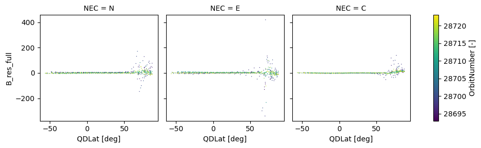
# Select one day
_ds = ds.sel({"Timestamp": slice("2019-01-01", "2019-01-02")})
# Select nightside data from it
_ds_dark = _ds.where(_ds["SunZenithAngle"] > 100, drop=True)
# Append a custom residual of B-MCO-MLI-MMA
_ds_dark["B_res_full"] = _ds_dark["B_NEC"] - _ds_dark["B_NEC_CHAOS-Core"] \
                                           - _ds_dark["B_NEC_CHAOS-Static"] \
                                           - _ds_dark["B_NEC_CHAOS-MMA-Primary"] \
                                           - _ds_dark["B_NEC_CHAOS-MMA-Secondary"]
_ds_dark.plot.scatter(x="QDLat", y="B_res_full", hue="OrbitNumber", col="NEC",
                      cmap="viridis", s=1, linewidths=0);

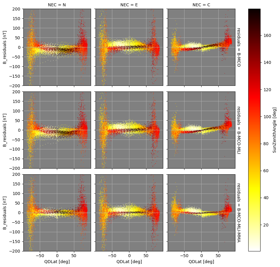
Residuals to model combinations (one month)

First we adjust the Dataset so that it contains the custom residuals themselves. We store them as both regular data variables and as a higher dimensional "B_residuals" which includes all of them. This is inefficient but is convenient for the plotting tools used below.

def assign_residuals(ds):
    # Work on a copy of the Dataset so we don't disturb the original
    ds = ds.copy()
    # Assign custom residual variables
    ds["B-MCO"] = ds["B_NEC"] - ds["B_NEC_CHAOS-Core"]
    ds["B-MCO-MLI"] = ds["B-MCO"] - ds["B_NEC_CHAOS-Static"]
    ds["B-MCO-MLI-MMA"] = ds["B-MCO-MLI"] - ds["B_NEC_CHAOS-MMA-Primary"]\
                                          - ds["B_NEC_CHAOS-MMA-Secondary"]
    # Create a new DataArray to contain all these residual combinations
    da = ds["B_NEC"].copy()
    da.name = "B_residuals"
    # Expand to 3 dimensions for each residual combination to use
    da = da.expand_dims({"residuals": 3})
    da.coords["residuals"] = ["B-MCO", "B-MCO-MLI", "B-MCO-MLI-MMA"]
    # Assign the residual data to the DataArray
    da = da.copy()
    da.loc[{"residuals": "B-MCO"}] = ds["B-MCO"]
    da.loc[{"residuals": "B-MCO-MLI"}] = ds["B-MCO-MLI"]
    da.loc[{"residuals": "B-MCO-MLI-MMA"}] = ds["B-MCO-MLI-MMA"]
    # Assign the new DataArray to the original Dataset
    ds["B_residuals"] = da
    return ds

ds = assign_residuals(ds)
ds

<xarray.Dataset>
Dimensions:                    (Timestamp: 242598, NEC: 3, residuals: 3)
Coordinates:
  * Timestamp                  (Timestamp) datetime64[ns] 2019-01-01 ... 2019...
  * NEC                        (NEC) <U1 'N' 'E' 'C'
  * residuals                  (residuals) <U13 'B-MCO' ... 'B-MCO-MLI-MMA'
Data variables: (12/17)
    Spacecraft                 (Timestamp) object 'A' 'A' 'A' ... 'A' 'A' 'A'
    MLT                        (Timestamp) float64 14.8 14.72 ... 6.219 6.348
    B_NEC_CHAOS-Static         (Timestamp, NEC) float64 -0.1243 1.575 ... 0.5559
    B_NEC_CHAOS-Core           (Timestamp, NEC) float64 2.369e+04 ... 4.915e+04
    B_NEC                      (Timestamp, NEC) float64 2.368e+04 ... 4.915e+04
    OrbitNumber                (Timestamp) int32 28692 28692 ... 34324 34324
    ...                         ...
    QDLat                      (Timestamp) float64 -13.95 -6.242 ... 57.39 64.82
    Longitude                  (Timestamp) float64 -136.0 -136.1 ... 97.65 99.22
    B-MCO                      (Timestamp, NEC) float64 -12.93 -19.23 ... 6.232
    B-MCO-MLI                  (Timestamp, NEC) float64 -12.81 -20.8 ... 5.676
    B-MCO-MLI-MMA              (Timestamp, NEC) float64 1.347 -22.79 ... -1.366
    B_residuals                (residuals, Timestamp, NEC) float64 -12.93 ......
Attributes:
    Sources:         Many
    MagneticModels:  ["CHAOS-Core = 'CHAOS-Core'(max_degree=20,min_degree=1)"...
    AppliedFilters:  ['Flags_F <= 1', 'Flags_F >= 0', 'Kp <= 3', 'Kp >= 0']

xarray.Dataset

• Dimensions:
  • Timestamp: 242598
  • NEC: 3
  • residuals: 3
• Coordinates: (3)
  • Timestamp
    (Timestamp)
    datetime64[ns]
    2019-01-01 ... 2019-12-31T23:58:00

    description :

    Time stamp

    array(['2019-01-01T00:00:00.000000000', '2019-01-01T00:02:00.000000000',
           '2019-01-01T00:04:00.000000000', ..., '2019-12-31T23:54:00.000000000',
           '2019-12-31T23:56:00.000000000', '2019-12-31T23:58:00.000000000'],
          dtype='datetime64[ns]')

  • NEC
    (NEC)
    <U1
    'N' 'E' 'C'

    units :

    description :

    NEC frame - North, East, Centre (down)

    array(['N', 'E', 'C'], dtype='<U1')

  • residuals
    (residuals)
    <U13
    'B-MCO' 'B-MCO-MLI' 'B-MCO-MLI-MMA'

    array(['B-MCO', 'B-MCO-MLI', 'B-MCO-MLI-MMA'], dtype='<U13')

• Data variables: (17)
  • Spacecraft
    (Timestamp)
    object
    'A' 'A' 'A' 'A' ... 'A' 'A' 'A' 'A'

    units :

    -

    description :

    Spacecraft identifier (values: 'A', 'B', 'C' or '-' if not available).

    array(['A', 'A', 'A', ..., 'A', 'A', 'A'], dtype=object)

  • MLT
    (Timestamp)
    float64
    14.8 14.72 14.65 ... 6.219 6.348

    units :

    h

    description :

    Magnetic local time

    array([14.79740524, 14.71789551, 14.65094757, ...,  6.12784386,
            6.21863174,  6.34835625])

  • B_NEC_CHAOS-Static
    (Timestamp, NEC)
    float64
    -0.1243 1.575 ... 2.338 0.5559

    units :

    nT

    description :

    Magnetic field vector, NEC frame, calculated by the CHAOS-Static spherical harmonic model

    array([[-0.12427424,  1.57504536, -0.36996116],
           [ 0.06280141,  0.72170757, -0.4087065 ],
           [ 0.17748272, -0.388705  ,  0.30508599],
           ...,
           [-0.47221455, -0.03294338, -0.95104102],
           [ 0.83005169, -1.69760825,  1.27594809],
           [ 1.93739102,  2.33844637,  0.55589511]])

  • B_NEC_CHAOS-Core
    (Timestamp, NEC)
    float64
    2.369e+04 5.314e+03 ... 4.915e+04

    units :

    nT

    description :

    Magnetic field vector, NEC frame, calculated by the CHAOS-Core spherical harmonic model

    array([[ 2.36889341e+04,  5.31437820e+03, -1.22471230e+04],
           [ 2.45843273e+04,  4.72325850e+03, -5.58645030e+03],
           [ 2.48485956e+04,  4.28227312e+03,  1.28326544e+03],
           ...,
           [ 1.40755929e+04, -4.19168816e+01,  4.66759050e+04],
           [ 9.73758897e+03,  1.20689105e+02,  4.86426646e+04],
           [ 6.01301505e+03,  2.72187878e+02,  4.91454266e+04]])

  • B_NEC
    (Timestamp, NEC)
    float64
    2.368e+04 5.295e+03 ... 4.915e+04

    units :

    nT

    description :

    Magnetic field vector, NEC frame

    array([[ 2.36760008e+04,  5.29515090e+03, -1.22484145e+04],
           [ 2.45740495e+04,  4.69856949e+03, -5.59765010e+03],
           [ 2.48499011e+04,  4.26006984e+03,  1.28627100e+03],
           ...,
           [ 1.40708616e+04, -4.05193482e+01,  4.66819932e+04],
           [ 9.73489373e+03,  1.19725402e+02,  4.86510680e+04],
           [ 6.01312094e+03,  2.77310333e+02,  4.91516582e+04]])

  • OrbitNumber
    (Timestamp)
    int32
    28692 28692 28692 ... 34324 34324

    units :

    -

    description :

    Orbit number (set to -1 if not available)

    array([28692, 28692, 28692, ..., 34324, 34324, 34324], dtype=int32)

  • Radius
    (Timestamp)
    float64
    6.819e+06 6.818e+06 ... 6.803e+06

    units :

    m

    description :

    Position in ITRF - Radius

    array([6819106.91, 6818073.77, 6816909.52, ..., 6805320.65, 6804302.47,
           6803498.32])

  • Latitude
    (Timestamp)
    float64
    -17.03 -9.329 ... 61.38 69.06

    units :

    deg

    description :

    Position in ITRF - Latitude

    array([-17.0299019,  -9.3287281,  -1.6242172, ...,  53.6733283,
            61.3772633,  69.0629806])

  • B_NEC_CHAOS-MMA-Secondary
    (Timestamp, NEC)
    float64
    -0.303 0.9856 ... -1.142 1.384

    units :

    nT

    description :

    Magnetic field vector, NEC frame, calculated by the CHAOS-MMA-Secondary spherical harmonic model

    array([[-0.30297056,  0.98564803, -2.89135236],
           [-0.10470823,  0.87585609, -2.91108254],
           [ 0.08722358,  0.76643363, -2.88592763],
           ...,
           [ 0.32726343, -1.21991201,  1.31986096],
           [ 0.16572226, -1.17265426,  1.38592177],
           [ 0.01670538, -1.14231647,  1.38397679]])

  • B_NEC_CHAOS-MMA-Primary
    (Timestamp, NEC)
    float64
    -13.85 1.0 1.269 ... -3.015 5.657

    units :

    nT

    description :

    Magnetic field vector, NEC frame, calculated by the CHAOS-MMA-Primary spherical harmonic model

    array([[-13.85326293,   1.00041826,   1.26932794],
           [-13.57361511,   0.72772099,   2.95157387],
           [-13.10998322,   0.45323748,   4.58952267],
           ...,
           [ -5.35689486,  -3.26147668,   4.64691082],
           [ -4.63973588,  -3.10838554,   5.19147355],
           [ -3.83557873,  -3.01480717,   5.65749524]])

  • SunZenithAngle
    (Timestamp)
    float64
    40.87 43.82 47.65 ... 107.4 108.7

    units :

    deg

    description :

    Sun position - zenith angle

    array([ 40.86874699,  43.82230911,  47.64623674, ..., 105.76064586,
           107.38050934, 108.68561163])

  • QDLat
    (Timestamp)
    float64
    -13.95 -6.242 1.515 ... 57.39 64.82

    units :

    deg

    description :

    Magnetic quasi-dipole latitude

    array([-13.95402908,  -6.24187136,   1.51521564, ...,  49.68329239,
            57.39051437,  64.82193756])

  • Longitude
    (Timestamp)
    float64
    -136.0 -136.1 ... 97.65 99.22

    units :

    deg

    description :

    Position in ITRF - Longitude

    array([-136.0207597, -136.1450285, -136.2855785, ...,   96.8970934,
             97.6468168,   99.2203183])

  • B-MCO
    (Timestamp, NEC)
    float64
    -12.93 -19.23 ... 5.122 6.232

    array([[-12.93328926, -19.22730367,  -1.29154661],
           [-10.27773072, -24.68900976, -11.19980436],
           [  1.30550781, -22.2032852 ,   3.00556135],
           ...,
           [ -4.73135199,   1.39753336,   6.08821302],
           [ -2.69523391,  -0.96370267,   8.40348281],
           [  0.10588504,   5.12245525,   6.23164093]])

  • B-MCO-MLI
    (Timestamp, NEC)
    float64
    -12.81 -20.8 ... 2.784 5.676

    array([[-12.80901501, -20.80234903,  -0.92158545],
           [-10.34053213, -25.41071733, -10.79109786],
           [  1.12802509, -21.8145802 ,   2.70047536],
           ...,
           [ -4.25913744,   1.43047674,   7.03925404],
           [ -3.52528559,   0.73390557,   7.12753472],
           [ -1.83150598,   2.78400888,   5.67574581]])

  • B-MCO-MLI-MMA
    (Timestamp, NEC)
    float64
    1.347 -22.79 ... 6.941 -1.366

    array([[  1.34721848, -22.78841532,   0.70043897],
           [  3.33779121, -27.01429441, -10.8315892 ],
           [ 14.15078473, -23.03425131,   0.99688032],
           ...,
           [  0.77049399,   5.91186543,   1.07248227],
           [  0.94872802,   5.01494537,   0.55013941],
           [  1.98736737,   6.94113253,  -1.36572622]])

  • B_residuals
    (residuals, Timestamp, NEC)
    float64
    -12.93 -19.23 ... 6.941 -1.366

    units :

    nT

    description :

    Magnetic field vector, NEC frame

    array([[[-12.93328926, -19.22730367,  -1.29154661],
            [-10.27773072, -24.68900976, -11.19980436],
            [  1.30550781, -22.2032852 ,   3.00556135],
            ...,
            [ -4.73135199,   1.39753336,   6.08821302],
            [ -2.69523391,  -0.96370267,   8.40348281],
            [  0.10588504,   5.12245525,   6.23164093]],
    
           [[-12.80901501, -20.80234903,  -0.92158545],
            [-10.34053213, -25.41071733, -10.79109786],
            [  1.12802509, -21.8145802 ,   2.70047536],
            ...,
            [ -4.25913744,   1.43047674,   7.03925404],
            [ -3.52528559,   0.73390557,   7.12753472],
            [ -1.83150598,   2.78400888,   5.67574581]],
    
           [[  1.34721848, -22.78841532,   0.70043897],
            [  3.33779121, -27.01429441, -10.8315892 ],
            [ 14.15078473, -23.03425131,   0.99688032],
            ...,
            [  0.77049399,   5.91186543,   1.07248227],
            [  0.94872802,   5.01494537,   0.55013941],
            [  1.98736737,   6.94113253,  -1.36572622]]])

• Indexes: (3)
  • Timestamp
    PandasIndex

    PandasIndex(DatetimeIndex(['2019-01-01 00:00:00', '2019-01-01 00:02:00',
                   '2019-01-01 00:04:00', '2019-01-01 00:06:00',
                   '2019-01-01 00:08:00', '2019-01-01 00:10:00',
                   '2019-01-01 00:12:00', '2019-01-01 00:14:00',
                   '2019-01-01 00:16:00', '2019-01-01 00:18:00',
                   ...
                   '2019-12-31 23:40:00', '2019-12-31 23:42:00',
                   '2019-12-31 23:44:00', '2019-12-31 23:46:00',
                   '2019-12-31 23:48:00', '2019-12-31 23:50:00',
                   '2019-12-31 23:52:00', '2019-12-31 23:54:00',
                   '2019-12-31 23:56:00', '2019-12-31 23:58:00'],
                  dtype='datetime64[ns]', name='Timestamp', length=242598, freq=None))

  • NEC
    PandasIndex

    PandasIndex(Index(['N', 'E', 'C'], dtype='object', name='NEC'))

  • residuals
    PandasIndex

    PandasIndex(Index(['B-MCO', 'B-MCO-MLI', 'B-MCO-MLI-MMA'], dtype='object', name='residuals'))

• Attributes: (3)

  Sources :

  Many

  MagneticModels :

  ["CHAOS-Core = 'CHAOS-Core'(max_degree=20,min_degree=1)", "CHAOS-MMA-Primary = 'CHAOS-MMA-Primary'(max_degree=2,min_degree=1)", "CHAOS-MMA-Secondary = 'CHAOS-MMA-Secondary'(max_degree=2,min_degree=1)", "CHAOS-Static = 'CHAOS-Static'(max_degree=185,min_degree=21)"]

  AppliedFilters :

  ['Flags_F <= 1', 'Flags_F >= 0', 'Kp <= 3', 'Kp >= 0']

Here we create scatter plots to show the data in different views. We select only the first month - this reduces the crowding on the figures but shows that we should seek different methods to produce summary views of the data for longer time periods.

facetgrid = (
    ds.sel({"Timestamp": slice("2019-01-01", "2019-02-01")})
      .plot.scatter(x="QDLat", y="B_residuals", col="NEC", row="residuals",
                    sharex="all", sharey="row", s=1, linewidths=0,
                    hue="SunZenithAngle", cmap="hot_r"))
for ax in facetgrid.axes.flat:
    ax.set_facecolor("grey")
    ax.grid()
    ax.set_ylim((-200, 200))

/tmp/ipykernel_2312/2614893674.py:6: DeprecationWarning: self.axes is deprecated since 2022.11 in order to align with matplotlibs plt.subplots, use self.axs instead.
  for ax in facetgrid.axes.flat:

(
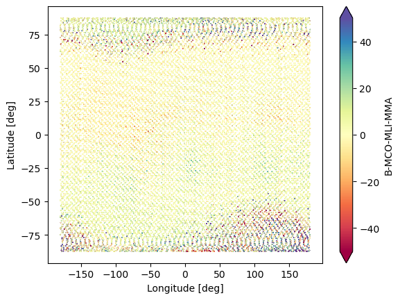
    ds
    .sel({"Timestamp": slice("2019-01-01", "2019-02-01")})
    .plot.scatter(x="Longitude", y="Latitude", hue="B-MCO-MLI-MMA",
                  s=1, linewidths=0, cmap="Spectral", vmin=-50, vmax=50)
);

(
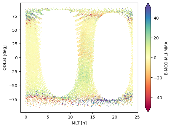
    ds
    .sel({"Timestamp": slice("2019-01-01", "2019-02-01")})
    .plot.scatter(x="MLT", y="QDLat", hue="B-MCO-MLI-MMA",
                  s=1, linewidths=0, cmap="Spectral", vmin=-50, vmax=50)
);

Statistical summaries of data over the full year

(
    ds
       .groupby_bins("QDLat", 90)
       .std()["B-MCO-MLI-MMA"]
       .plot.line(x="QDLat_bins")
)
plt.suptitle("Standard deviations");

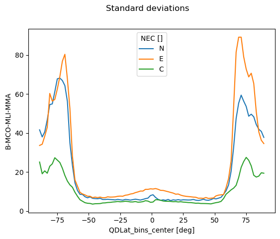
This shows the large variability in the data over the polar regions