EFIxTCT (Cross-track ion flow)#
Abstract: Access to the 2Hz & 16Hz cross-track ion flow data derived from the Thermal Ion Imager (TII), part of the Electric Field Instrument package (EFI).
Documentation:
# Display important package versions used
%load_ext watermark
%watermark -i -v -p viresclient,pandas,xarray,matplotlib
Python implementation: CPython
Python version       : 3.11.6
IPython version      : 8.18.0

viresclient: 0.15.0
pandas     : 2.1.3
xarray     : 2023.12.0
matplotlib : 3.8.2
import matplotlib as mpl
import matplotlib.pyplot as plt
import numpy as np
import xarray as xr

# Control the HTML display of the datasets
xr.set_options(
    display_expand_attrs=False, display_expand_coords=True, display_expand_data=True
)

from viresclient import SwarmRequest
request = SwarmRequest()
What data is available?#
There are two sets of collections available, one for 2Hz and one for 16Hz, and for each there are three collections, one for each Swarm spacecraft.
request.available_collections("EFI_TCT02", details=False)
{'EFI_TCT02': ['SW_EXPT_EFIA_TCT02',
  'SW_EXPT_EFIB_TCT02',
  'SW_EXPT_EFIC_TCT02']}
request.available_collections("EFI_TCT16", details=False)
{'EFI_TCT16': ['SW_EXPT_EFIA_TCT16',
  'SW_EXPT_EFIB_TCT16',
  'SW_EXPT_EFIC_TCT16']}
print(request.available_measurements("EFI_TCT02"))
['VsatC', 'VsatE', 'VsatN', 'Bx', 'By', 'Bz', 'Ehx', 'Ehy', 'Ehz', 'Evx', 'Evy', 'Evz', 'Vicrx', 'Vicry', 'Vicrz', 'Vixv', 'Vixh', 'Viy', 'Viz', 'Vixv_error', 'Vixh_error', 'Viy_error', 'Viz_error', 'Latitude_QD', 'MLT_QD', 'Calibration_flags', 'Quality_flags']
print(request.available_measurements("EFI_TCT16"))
['VsatC', 'VsatE', 'VsatN', 'Bx', 'By', 'Bz', 'Ehx', 'Ehy', 'Ehz', 'Evx', 'Evy', 'Evz', 'Vicrx', 'Vicry', 'Vicrz', 'Vixv', 'Vixh', 'Viy', 'Viz', 'Vixv_error', 'Vixh_error', 'Viy_error', 'Viz_error', 'Latitude_QD', 'MLT_QD', 'Calibration_flags', 'Quality_flags']
As seen above, the variables available for both the 2Hz and 16Hz datasets are the same. Here is a short description for each variable:
tct_vars = [
    # Satellite velocity in NEC frame
    "VsatC",
    "VsatE",
    "VsatN",
    # Geomagnetic field components derived from 1Hz product
    #  (in satellite-track coordinates)
    "Bx",
    "By",
    "Bz",
    # Electric field components derived from -VxB with along-track ion drift
    #  (in satellite-track coordinates)
    # Eh: derived from horizontal sensor
    # Ev: derived from vertical sensor
    "Ehx",
    "Ehy",
    "Ehz",
    "Evx",
    "Evy",
    "Evz",
    # Ion drift corotation signal, removed from ion drift & electric field
    #  (in satellite-track coordinates)
    "Vicrx",
    "Vicry",
    "Vicrz",
    # Ion drifts along-track from vertical (..v) and horizontal (..h) TII sensor
    "Vixv",
    "Vixh",
    # Ion drifts cross-track (y from horizontal sensor, z from vertical sensor)
    #  (in satellite-track coordinates)
    "Viy",
    "Viz",
    # Random error estimates for the above
    #  (Negative value indicates no estimate available)
    "Vixv_error",
    "Vixh_error",
    "Viy_error",
    "Viz_error",
    # Quasi-dipole magnetic latitude and local time
    #  redundant with VirES auxiliaries, QDLat & MLT
    "Latitude_QD",
    "MLT_QD",
    # Refer to release notes link above for details:
    "Calibration_flags",
    "Quality_flags",
]
Fetching and plotting data#
For demonstration, we will fetch the 2Hz data from Swarm Alpha (SW_EXPT_EFIA_TCT02)
start = "2018-07-17T11:00:00"
end = "2018-07-17T16:00:00"

request = SwarmRequest()
request.set_collection("SW_EXPT_EFIA_TCT02")
request.set_products(measurements=tct_vars)
data = request.get_between(start, end)
Data can be loaded as either a pandas datframe or a xarray dataset.
df = data.as_dataframe()
df.head()
| VsatN | Vixh | Ehy | Calibration_flags | Spacecraft | Longitude | Ehz | Bx | Vixv | Radius | ... | Ehx | Quality_flags | Vicrx | Viy_error | Evz | Latitude_QD | Evx | Viz | Bz | Vicrz | |
|---|---|---|---|---|---|---|---|---|---|---|---|---|---|---|---|---|---|---|---|---|---|
| Timestamp | |||||||||||||||||||||
| 2018-07-17 11:28:49.231500032 | -7367.485352 | -4369.472168 | -208.541107 | 50529027 | A | 83.452042 | -13.000871 | -1941.969727 | -6378.091797 | 6805732.5 | ... | -101.939255 | 0 | -19.133141 | -14.849242 | -17.083946 | 75.221916 | -101.939255 | 240.197159 | 47833.585938 | -0.658330 |
| 2018-07-17 11:28:49.731500032 | -7369.272461 | -4536.605469 | -216.759445 | 50529027 | A | 83.500351 | -13.498644 | -1947.767822 | -6341.005371 | 6805734.5 | ... | -105.307312 | 0 | -19.119896 | -14.849242 | -17.166695 | 75.193153 | -105.307312 | 134.010635 | 47837.687500 | -0.661254 |
| 2018-07-17 11:28:50.231500032 | -7371.040527 | -4604.627441 | -220.021118 | 50529027 | A | 83.548347 | -13.564169 | -1954.280518 | -6508.682617 | 6805735.5 | ... | -103.137848 | 0 | -19.106642 | -14.849242 | -17.435713 | 75.164375 | -103.137848 | 139.632843 | 47841.738281 | -0.664178 |
| 2018-07-17 11:28:50.731500032 | -7372.794922 | -4507.862793 | -215.698181 | 50529027 | A | 83.596039 | -13.433209 | -1961.330688 | -6535.101562 | 6805736.0 | ... | -103.988091 | 0 | -19.093380 | -14.849242 | -17.556908 | 75.135590 | -103.988091 | -8.017212 | 47845.742188 | -0.667102 |
| 2018-07-17 11:28:51.231500032 | -7374.530762 | -4699.985352 | -224.552765 | 50529027 | A | 83.643425 | -13.663168 | -1969.853027 | -6356.244629 | 6805737.0 | ... | -100.248749 | 0 | -19.080120 | -14.849242 | -17.029562 | 75.106796 | -100.248749 | 172.994843 | 47849.816406 | -0.670023 |
5 rows × 31 columns
ds = data.as_xarray()
ds
<xarray.Dataset>
Dimensions:            (Timestamp: 32535)
Coordinates:
  * Timestamp          (Timestamp) datetime64[ns] 2018-07-17T11:28:49.2315000...
Data variables: (12/31)
    Spacecraft         (Timestamp) object 'A' 'A' 'A' 'A' ... 'A' 'A' 'A' 'A'
    Vixh               (Timestamp) float32 -4.369e+03 -4.537e+03 ... -4.744e+03
    Ehy                (Timestamp) float32 -208.5 -216.8 ... -209.6 -206.1
    Longitude          (Timestamp) float32 83.45 83.5 83.55 ... -143.5 -143.5
    Ehz                (Timestamp) float32 -13.0 -13.5 -13.56 ... 23.66 22.61
    Radius             (Timestamp) float32 6.806e+06 6.806e+06 ... 6.807e+06
    ...                 ...
    MLT_QD             (Timestamp) float32 17.15 17.15 17.16 ... 4.769 4.769
    Vixh_error         (Timestamp) float32 -14.85 -14.85 ... -14.85 -14.85
    Viy                (Timestamp) float32 2.121e+03 2.196e+03 ... 1.317e+03
    Vixv_error         (Timestamp) float32 -14.85 -14.85 ... -14.85 -14.85
    Viy_error          (Timestamp) float32 -14.85 -14.85 ... -14.85 -14.85
    Latitude_QD        (Timestamp) float32 75.22 75.19 75.16 ... 65.81 65.84
Attributes: (3)An example plot:
fig, axes = plt.subplots(nrows=4, sharex=True, figsize=(10, 7))
# Plot velocities with left axis
ds.plot.scatter(x="Timestamp", y="Vixv", ax=axes[0], s=1, linewidths=0)
ds.plot.scatter(x="Timestamp", y="Vixh", ax=axes[1], s=1, linewidths=0)
ds.plot.scatter(x="Timestamp", y="Viy", ax=axes[2], s=1, linewidths=0)
ds.plot.scatter(
    x="Timestamp", y="Viz", ax=axes[3], s=1, linewidths=0, label="Velocities"
)
# Plot velocities with right axis
axes_r = [ax.twinx() for ax in axes]
ds.plot.scatter(x="Timestamp", y="Vixv_error", ax=axes_r[0], s=0.1, color="tab:orange")
ds.plot.scatter(x="Timestamp", y="Vixh_error", ax=axes_r[1], s=0.1, color="tab:orange")
ds.plot.scatter(x="Timestamp", y="Viy_error", ax=axes_r[2], s=0.1, color="tab:orange")
ds.plot.scatter(x="Timestamp", y="Viz_error", ax=axes_r[3], s=0.1, color="tab:orange")
fig.subplots_adjust(hspace=0)
# Add legend to identify each side
blue = mpl.patches.Patch(color="tab:blue", label="Velocities")
orange = mpl.patches.Patch(color="tab:orange", label="Errors")
axes[0].legend(handles=[blue, orange])
# # Generate additional ticklabels for x-axis
# Use time xticks to get dataset vars at those xticks
locx = axes[-1].get_xticks()
times = mpl.dates.num2date(locx)
times = [t.replace(tzinfo=None) for t in times]
_ds_xticks = ds.reindex({"Timestamp": times}, method="nearest")
# Build ticklabels from dataset vars
xticklabels = np.stack(
    [
        _ds_xticks["Timestamp"].dt.strftime("%H:%M").values,
        np.round(_ds_xticks["Latitude"].values, 2).astype(str),
        np.round(_ds_xticks["Longitude"].values, 2).astype(str),
    ]
)
xticklabels = ["\n".join(row) for row in xticklabels.T]
# Add labels to first xtick
_xt0 = xticklabels[0].split("\n")
xticklabels[0] = f"Time:  {_xt0[0]}\nLat:  {_xt0[1]}\nLon: {_xt0[2]}"
axes[-1].set_xticks(axes[-1].get_xticks())
axes[-1].set_xticklabels(xticklabels)
axes[-1].set_xlabel("")
# Adjust title
title = "".join(
    [
        f"Swarm {ds['Spacecraft'].data[0]} 2Hz ion flow, ",
        ds["Timestamp"].dt.date.data[0].isoformat(),
        f"\n{ds.attrs['Sources']}",
    ]
)
fig.suptitle(title);
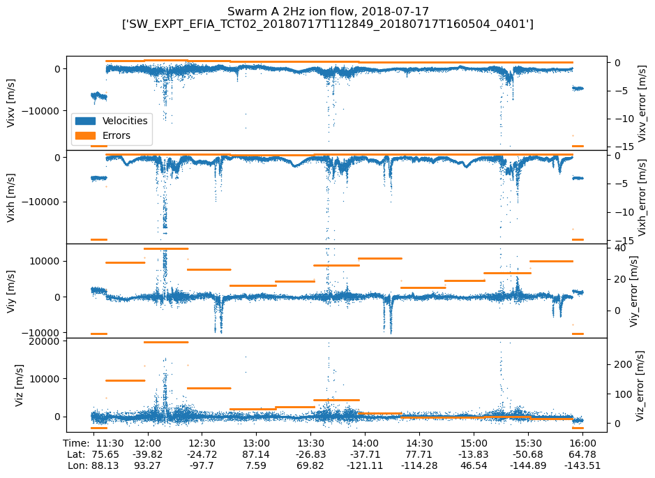
Due to contamination in the instrument, great care must be taken to use these data correctly. Check the release notes and make use of the Quality_flags variable to identify valid data periods.
TODO: use section 3.4.1.1 to identify untrusty periods (bitx = 0) and shade them grey?