AOBxFAC (Auroral oval boundaries)

Abstract: Access to the AEBS project output, boundaries of the auroral oval determined from field-aligned currents

See also:

• https://nbviewer.jupyter.org/github/pacesm/jupyter_notebooks/blob/master/AEBS/AEBS_AOB_FAC.ipynb

• https://earth.esa.int/eogateway/search?filter=swarm&text=aebs

Accessing the collection

from viresclient import SwarmRequest
import datetime as dt
import matplotlib.pyplot as plt

request = SwarmRequest()
request.available_collections("AOB_FAC", details=False)

{'AOB_FAC': ['SW_OPER_AOBAFAC_2F', 'SW_OPER_AOBBFAC_2F', 'SW_OPER_AOBCFAC_2F']}

request.available_measurements("AOB_FAC")

['Latitude_QD',
 'Longitude_QD',
 'MLT_QD',
 'Boundary_Flag',
 'Quality',
 'Pair_Indicator']

Let’s fetch one month of measurements. We will also fetch magnetic coordinates and the orbit direction flag for extra context, which we will use later in the figure.

request.set_collection("SW_OPER_AOBAFAC_2F")
request.set_products(
    ['Latitude_QD',
     'Longitude_QD',
     'MLT_QD',
     'Boundary_Flag',
     'Quality',
     'Pair_Indicator'],
    auxiliaries=["QDOrbitDirection", "QDLat", "QDLon", "MLT"]
)
data = request.get_between(
    dt.datetime(2016, 1, 1),
    dt.datetime(2016, 2, 1)
)

ds = data.as_xarray()
# Remove the Sources attribute now to keep the notebook cleaner
ds.attrs.pop("Sources")
ds

<xarray.Dataset>
Dimensions:           (Timestamp: 3157, Quality_dim1: 2)
Coordinates:
  * Timestamp         (Timestamp) datetime64[ns] 2016-01-01T00:07:01.500000 ....
Dimensions without coordinates: Quality_dim1
Data variables: (12/14)
    Spacecraft        (Timestamp) object 'A' 'A' 'A' 'A' 'A' ... 'A' 'A' 'A' 'A'
    MLT_QD            (Timestamp) float64 18.61 18.04 17.11 ... 1.216 0.2201
    QDLon             (Timestamp) float64 -5.015 -14.53 -36.0 ... 99.16 83.28
    Radius            (Timestamp) float64 6.834e+06 6.834e+06 ... 6.834e+06
    Pair_Indicator    (Timestamp) int8 1 -1 1 -1 1 -1 1 -1 ... -1 1 -1 1 -1 1 -1
    Longitude_QD      (Timestamp) float64 -5.015 -14.53 -36.0 ... 99.16 83.28
    ...                ...
    QDOrbitDirection  (Timestamp) int8 1 1 1 1 -1 -1 -1 -1 ... 1 1 1 -1 -1 -1 -1
    MLT               (Timestamp) float64 18.61 18.04 17.11 ... 1.216 0.2201
    Quality           (Timestamp, Quality_dim1) float64 3.572 0.1437 ... 0.2844
    QDLat             (Timestamp) float64 -67.88 -53.31 56.62 ... -57.92 -68.26
    Boundary_Flag     (Timestamp) uint8 2 1 1 2 2 1 1 2 2 ... 2 2 1 1 2 2 1 1 2
    Latitude          (Timestamp) float64 -80.0 -64.82 48.04 ... -53.34 -67.73
Attributes:
    MagneticModels:  []
    AppliedFilters:  []

xarray.Dataset

• Dimensions:
  • Timestamp: 3157
  • Quality_dim1: 2
• Coordinates: (1)
  • Timestamp
    (Timestamp)
    datetime64[ns]
    2016-01-01T00:07:01.500000 ... 2...

    description :

    Time of observation, UTC

    array(['2016-01-01T00:07:01.500000000', '2016-01-01T00:11:02.500000000',
           '2016-01-01T00:40:26.500000000', ..., '2016-01-31T23:23:04.500000000',
           '2016-01-31T23:52:45.500000000', '2016-01-31T23:56:31.500000000'],
          dtype='datetime64[ns]')

• Data variables: (14)
  • Spacecraft
    (Timestamp)
    object
    'A' 'A' 'A' 'A' ... 'A' 'A' 'A' 'A'

    units :

    -

    description :

    Spacecraft identifier (values: 'A', 'B', 'C' or '-' if not available).

    array(['A', 'A', 'A', ..., 'A', 'A', 'A'], dtype=object)

  • MLT_QD
    (Timestamp)
    float64
    18.61 18.04 17.11 ... 1.216 0.2201

    units :

    description :

    Magnetic Local Time (QD)

    array([18.60910034, 18.04205322, 17.10720253, ...,  2.28692436,
            1.21640396,  0.22005653])

  • QDLon
    (Timestamp)
    float64
    -5.015 -14.53 -36.0 ... 99.16 83.28

    units :

    deg

    description :

    Magnetic quasi-dipole longitude

    array([ -5.01492786, -14.53096199, -35.99659348, ..., 122.57527924,
            99.16169739,  83.27895355])

  • Radius
    (Timestamp)
    float64
    6.834e+06 6.834e+06 ... 6.834e+06

    units :

    description :

    Position in ITRF - Geocentric radius (from the Earth center)

    array([6834033.305, 6833848.575, 6819847.66 , ..., 6816024.46 ,
           6833355.3  , 6834007.43 ])

  • Pair_Indicator
    (Timestamp)
    int8
    1 -1 1 -1 1 -1 1 ... 1 -1 1 -1 1 -1

    units :

    description :

    Indicator of equatorward/poleward boundary of auroral oval. If the auroral oval boundaries are detectable as one pair, the pair indicator represents the record of previous (-1) or next (1) equatorward/poleward boundary within one pair; otherwise, the pair indicator is set to 0

    array([ 1, -1,  1, ..., -1,  1, -1], dtype=int8)

  • Longitude_QD
    (Timestamp)
    float64
    -5.015 -14.53 -36.0 ... 99.16 83.28

    units :

    description :

    Quasi-dipole longitude

    array([ -5.01492834, -14.53096199, -35.99659348, ..., 122.57541656,
            99.16161346,  83.27884674])

  • Longitude
    (Timestamp)
    float64
    -112.7 -104.1 ... 47.91 49.89

    units :

    description :

    Position in ITRF - Geocentric longitude

    array([-112.68401315, -104.09762171, -102.85523662, ...,   47.05311951,
             47.90735691,   49.88606176])

  • Latitude_QD
    (Timestamp)
    float64
    -67.88 -53.31 ... -57.92 -68.26

    units :

    description :

    Quasi-dipole latitude

    array([-67.87869263, -53.30882645,  56.62130356, ...,  57.02433395,
           -57.91941833, -68.25691986])

  • QDOrbitDirection
    (Timestamp)
    int8
    1 1 1 1 -1 -1 ... 1 1 -1 -1 -1 -1

    units :

    -

    description :

    Orbit direction in magnetic (QD) coordinates (values: 1 - ascending, -1 - descending, 0 - undefined)

    array([ 1,  1,  1, ..., -1, -1, -1], dtype=int8)

  • MLT
    (Timestamp)
    float64
    18.61 18.04 17.11 ... 1.216 0.2201

    units :

    h

    description :

    Magnetic local time

    array([18.60910034, 18.04205322, 17.10720253, ...,  2.28691483,
            1.21641159,  0.22006416])

  • Quality
    (Timestamp, Quality_dim1)
    float64
    3.572 0.1437 1.687 ... 2.965 0.2844

    units :

    description :

    Quality indicator of equatorward/poleward boundary (Pa, Sigma)

    array([[3.57207237, 0.14369166],
           [1.68731322, 0.21852749],
           [0.9336876 , 0.35753697],
           ...,
           [0.68972148, 0.30307527],
           [1.06752371, 0.19414563],
           [2.96545343, 0.28442717]])

  • QDLat
    (Timestamp)
    float64
    -67.88 -53.31 ... -57.92 -68.26

    units :

    deg

    description :

    Magnetic quasi-dipole latitude

    array([-67.87869263, -53.30882645,  56.62130356, ...,  57.02444839,
           -57.91941452, -68.25694275])

  • Boundary_Flag
    (Timestamp)
    uint8
    2 1 1 2 2 1 1 2 ... 2 1 1 2 2 1 1 2

    units :

    description :

    Indicator for equatorward (=1) or poleward (=2) boundary

    array([2, 1, 1, ..., 1, 1, 2], dtype=uint8)

  • Latitude
    (Timestamp)
    float64
    -80.0 -64.82 ... -53.34 -67.73

    units :

    description :

    Position in ITRF - Geocentric latitude

    array([-80.00245575, -64.81824633,  48.04237328, ...,  60.70888964,
           -53.34025313, -67.72552436])

• Indexes: (1)
  • Timestamp
    PandasIndex

    PandasIndex(DatetimeIndex(['2016-01-01 00:07:01.500000', '2016-01-01 00:11:02.500000',
                   '2016-01-01 00:40:26.500000', '2016-01-01 00:42:37.500000',
                   '2016-01-01 00:54:10.500000', '2016-01-01 00:58:31.500000',
                   '2016-01-01 01:27:29.500000', '2016-01-01 01:31:22.500000',
                   '2016-01-01 01:42:11.500000', '2016-01-01 01:45:40.500000',
                   ...
                   '2016-01-31 22:17:52.500000', '2016-01-31 22:21:16.500000',
                   '2016-01-31 22:31:28.500000', '2016-01-31 22:33:52.500000',
                   '2016-01-31 23:07:12.500000', '2016-01-31 23:09:11.500000',
                   '2016-01-31 23:19:39.500000', '2016-01-31 23:23:04.500000',
                   '2016-01-31 23:52:45.500000', '2016-01-31 23:56:31.500000'],
                  dtype='datetime64[ns]', name='Timestamp', length=3157, freq=None))

• Attributes: (2)

  MagneticModels :

  []

  AppliedFilters :

  []

Visualising the data

We can filter out for orbital segments where the spacecraft is approaching the pole (i.e. roughly within the same local time sector) using the QDOrbitDirection flag, and identify only the equatorward boundaries of the detected auroral oval using the Boundary_Flag like so:

ds.where(
    (ds["Boundary_Flag"]==1) & (ds["QDOrbitDirection"] == 1) & (ds["Latitude"] < 0)
).dropna(dim="Timestamp")["QDLat"].plot.line(x="Timestamp");

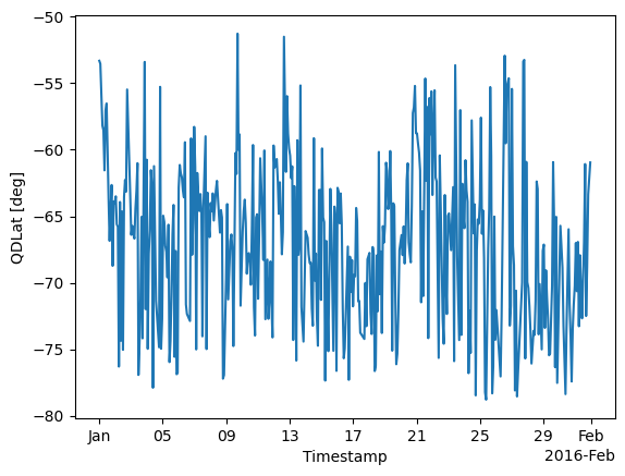
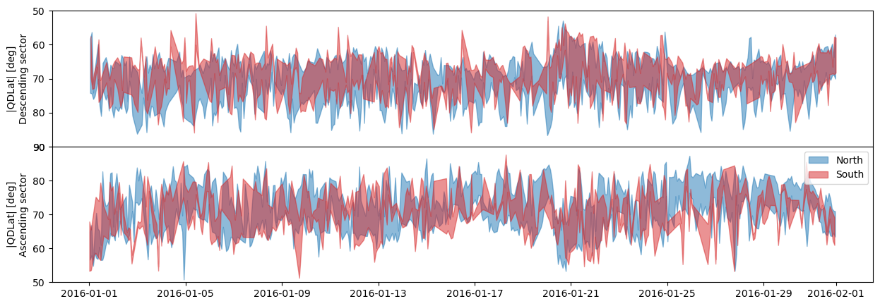
That shows us one edge of the auroral oval. Now let’s expand this idea to show both edges (filling between them), for both sectors of the auroral oval crossing (toward and away from the pole), for both Northern and Southern hemispheres.

ds = ds.where(ds["Pair_Indicator"] != 0)

northern_poleward_boundaries_ascendingsector = ds.where(
    (ds["Latitude"] > 0) & (ds["Boundary_Flag"] == 2) & (ds["QDOrbitDirection"] == 1)
).dropna(dim="Timestamp")
northern_equatorward_boundaries_ascendingsector = ds.where(
    (ds["Latitude"] > 0) & (ds["Boundary_Flag"] == 1) & (ds["QDOrbitDirection"] == 1)
).dropna(dim="Timestamp")

northern_poleward_boundaries_descendingsector = ds.where(
    (ds["Latitude"] > 0) & (ds["Boundary_Flag"] == 2) & (ds["QDOrbitDirection"] == -1)
).dropna(dim="Timestamp")
northern_equatorward_boundaries_descendingsector = ds.where(
    (ds["Latitude"] > 0) & (ds["Boundary_Flag"] == 1) & (ds["QDOrbitDirection"] == -1)
).dropna(dim="Timestamp")

southern_poleward_boundaries_ascendingsector = ds.where(
    (ds["Latitude"] < 0) & (ds["Boundary_Flag"] == 2) & (ds["QDOrbitDirection"] == 1)
).dropna(dim="Timestamp")
southern_equatorward_boundaries_ascendingsector = ds.where(
    (ds["Latitude"] < 0) & (ds["Boundary_Flag"] == 1) & (ds["QDOrbitDirection"] == 1)
).dropna(dim="Timestamp")

southern_poleward_boundaries_descendingsector = ds.where(
    (ds["Latitude"] < 0) & (ds["Boundary_Flag"] == 2) & (ds["QDOrbitDirection"] == -1)
).dropna(dim="Timestamp")
southern_equatorward_boundaries_descendingsector = ds.where(
    (ds["Latitude"] < 0) & (ds["Boundary_Flag"] == 1) & (ds["QDOrbitDirection"] == -1)
).dropna(dim="Timestamp")

fig, axes = plt.subplots(nrows=2, ncols=1, figsize=(15, 5), sharex=True)
axes[0].fill_between(
    x=northern_equatorward_boundaries_descendingsector["Timestamp"],
    y1=northern_equatorward_boundaries_descendingsector["QDLat"],
    y2=northern_poleward_boundaries_descendingsector["QDLat"],
    color="tab:blue",
    alpha=0.5
)
axes[0].fill_between(
    x=southern_equatorward_boundaries_descendingsector["Timestamp"],
    y1=-southern_equatorward_boundaries_descendingsector["QDLat"],
    y2=-southern_poleward_boundaries_descendingsector["QDLat"],
    color="tab:red",
    alpha=0.5
)

axes[1].fill_between(
    x=northern_equatorward_boundaries_ascendingsector["Timestamp"],
    y1=northern_equatorward_boundaries_ascendingsector["QDLat"],
    y2=northern_poleward_boundaries_ascendingsector["QDLat"],
    color="tab:blue",
    alpha=0.5,
    label="North"
)
axes[1].fill_between(
    x=southern_equatorward_boundaries_ascendingsector["Timestamp"],
    y1=-southern_equatorward_boundaries_ascendingsector["QDLat"],
    y2=-southern_poleward_boundaries_ascendingsector["QDLat"],
    color="tab:red",
    alpha=0.5,
    label="South"
)

axes[0].set_ylim((90, 50))
axes[1].set_ylim((50, 90))
fig.subplots_adjust(hspace=0)
axes[1].set_ylabel("|QDLat| [deg]\nAscending sector");
axes[0].set_ylabel("|QDLat| [deg]\nDescending sector");
axes[1].legend();

TODO

• Only fill between times where well determined (break up into segments which are contiguous and do many sequential fill_between’s)