EFIx_LP_1B (Langmuir probe 2Hz)

Abstract: Access to the electric field instrument langmuir probe data (2Hz) (level 1b product).

%load_ext watermark
%watermark -i -v -p viresclient,pandas,xarray,matplotlib

Python implementation: CPython
Python version       : 3.11.6
IPython version      : 8.18.0

viresclient: 0.15.0
pandas     : 2.1.3
xarray     : 2023.12.0
matplotlib : 3.8.2

import datetime as dt

import matplotlib.pyplot as plt
from viresclient import SwarmRequest

request = SwarmRequest()

EFIx_LP_1B product information

Measurements from the Langmuir Probe (LP) of the Electric Field Instrument (EFI) at 2Hz, for each Swarm spacecraft.

Documentation:

• https://earth.esa.int/web/guest/missions/esa-eo-missions/swarm/data-handbook/level-1b-product-definitions#EFIX_LP_1B_Product

Check what “EFI” data variables are available

request.available_collections("EFI", details=False)

{'EFI': ['SW_OPER_EFIA_LP_1B', 'SW_OPER_EFIB_LP_1B', 'SW_OPER_EFIC_LP_1B']}

request.available_measurements("EFI")

['U_orbit',
 'N_ion',
 'dN_ion',
 'N_ion_error',
 'N_elec',
 'N_elec_error',
 'T_elec',
 'dT_elec',
 'T_elec_error',
 'Vs',
 'Vs_error',
 'Flags_N_elec',
 'Flags_N_ion',
 'Flags_T_elec',
 'Flags_Vs',
 'Flagbits1',
 'Flagbits2',
 'Gamma1',
 'Gamma2']

Fetch one day of EFI data

request.set_collection("SW_OPER_EFIA_LP_1B")
request.set_products(
    measurements=[
        "U_orbit",
        "N_ion",
        "dN_ion",
        "T_elec",
        "dT_elec",
        "Vs",
        "Vs_error",
        "Flags_N_ion",
        "Flags_T_elec",
        "Flags_Vs",
    ]
)
data = request.get_between(dt.datetime(2016, 1, 1), dt.datetime(2016, 1, 2))

data.sources

['SW_OPER_EFIA_LP_1B_20160101T000000_20160101T235959_0701_MDR_EFI_LP']

Load and plot using pandas/matplotlib

df = data.as_dataframe()
df.head()

	T_elec	Radius	dT_elec	Flags_Vs	Latitude	U_orbit	Flags_T_elec	Vs	Flags_N_ion	Vs_error	dN_ion	Longitude	N_ion	Spacecraft
Timestamp
2016-01-01 00:00:00.196999936	2945.204213	6833853.41	-245.895850	20	-72.511716	7604.407	20	-2.201	20	NaN	28365.234486	92.799630	126188.350497	A
2016-01-01 00:00:00.696000000	2891.969742	6833854.00	-259.711123	20	-72.543238	7604.397	20	-2.193	20	NaN	28725.923124	92.813943	127792.945177	A
2016-01-01 00:00:01.196999936	2921.955198	6833854.59	-247.826218	20	-72.574886	7604.388	20	-2.200	20	NaN	29787.432673	92.828370	132515.280154	A
2016-01-01 00:00:01.696000000	2936.736557	6833855.18	-239.714158	20	-72.606406	7604.379	20	-2.194	20	NaN	31005.243307	92.842799	137932.951397	A
2016-01-01 00:00:02.196999936	2870.090847	6833855.77	-257.759606	20	-72.638051	7604.370	20	-2.190	20	NaN	31225.718904	92.857342	138913.780654	A

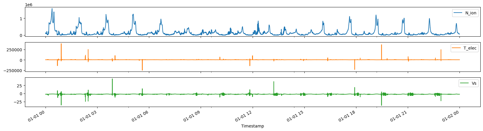
df.plot(y=["N_ion", "T_elec", "Vs"], subplots=True, figsize=(20,5));

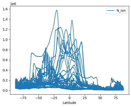
df.plot(x="Latitude", y="N_ion");

Load as xarray

ds = data.as_xarray()
ds

<xarray.Dataset>
Dimensions:       (Timestamp: 172776)
Coordinates:
  * Timestamp     (Timestamp) datetime64[ns] 2016-01-01T00:00:00.196999936 .....
Data variables: (12/14)
    Spacecraft    (Timestamp) object 'A' 'A' 'A' 'A' 'A' ... 'A' 'A' 'A' 'A' 'A'
    T_elec        (Timestamp) float64 2.945e+03 2.892e+03 ... 2.545e+03
    Radius        (Timestamp) float64 6.834e+06 6.834e+06 ... 6.823e+06
    dT_elec       (Timestamp) float64 -245.9 -259.7 -247.8 ... -408.5 -403.6
    Flags_Vs      (Timestamp) uint8 20 20 20 20 20 20 20 ... 20 20 20 20 20 20
    Latitude      (Timestamp) float64 -72.51 -72.54 -72.57 ... 31.65 31.69 31.72
    ...            ...
    Vs            (Timestamp) float64 -2.201 -2.193 -2.2 ... -2.239 -2.243
    Flags_N_ion   (Timestamp) uint8 20 20 20 20 20 20 20 ... 20 20 20 20 20 20
    Vs_error      (Timestamp) float64 nan nan nan nan nan ... nan nan nan nan
    dN_ion        (Timestamp) float64 2.837e+04 2.873e+04 ... 1.445e+04
    Longitude     (Timestamp) float64 92.8 92.81 92.83 ... -95.37 -95.37 -95.37
    N_ion         (Timestamp) float64 1.262e+05 1.278e+05 ... 6.485e+04 6.43e+04
Attributes:
    Sources:         ['SW_OPER_EFIA_LP_1B_20160101T000000_20160101T235959_070...
    MagneticModels:  []
    AppliedFilters:  []

xarray.Dataset

• Dimensions:
  • Timestamp: 172776
• Coordinates: (1)
  • Timestamp
    (Timestamp)
    datetime64[ns]
    2016-01-01T00:00:00.196999936 .....

    description :

    Time stamp

    array(['2016-01-01T00:00:00.196999936', '2016-01-01T00:00:00.696000000',
           '2016-01-01T00:00:01.196999936', ..., '2016-01-01T23:59:58.696000000',
           '2016-01-01T23:59:59.196999936', '2016-01-01T23:59:59.696000000'],
          dtype='datetime64[ns]')

• Data variables: (14)
  • Spacecraft
    (Timestamp)
    object
    'A' 'A' 'A' 'A' ... 'A' 'A' 'A' 'A'

    units :

    -

    description :

    Spacecraft identifier (values: 'A', 'B', 'C' or '-' if not available).

    array(['A', 'A', 'A', ..., 'A', 'A', 'A'], dtype=object)

  • T_elec
    (Timestamp)
    float64
    2.945e+03 2.892e+03 ... 2.545e+03

    units :

    K

    description :

    Plasma electron temperature

    array([2945.20421293, 2891.96974223, 2921.95519825, ..., 2568.06791336,
           2526.61671558, 2545.17018937])

  • Radius
    (Timestamp)
    float64
    6.834e+06 6.834e+06 ... 6.823e+06

    units :

    m

    description :

    Position in ITRF - Radius

    array([6833853.41, 6833854.  , 6833854.59, ..., 6822824.68, 6822821.24,
           6822821.74])

  • dT_elec
    (Timestamp)
    float64
    -245.9 -259.7 ... -408.5 -403.6

    units :

    cm-3

    description :

    Suggested calibration correction od T_elec

    array([-245.89585004, -259.71112264, -247.82621788, ..., -396.96304581,
           -408.46046478, -403.64152422])

  • Flags_Vs
    (Timestamp)
    uint8
    20 20 20 20 20 ... 20 20 20 20 20

    units :

    -

    description :

    Flags characterizing the spacecraft potential measurement

    array([20, 20, 20, ..., 20, 20, 20], dtype=uint8)

  • Latitude
    (Timestamp)
    float64
    -72.51 -72.54 ... 31.69 31.72

    units :

    deg

    description :

    Position in ITRF - Latitude

    array([-72.5117157, -72.5432384, -72.5748862, ...,  31.6548053,
            31.6869228,  31.7189122])

  • U_orbit
    (Timestamp)
    float64
    7.604e+03 7.604e+03 ... 7.634e+03

    units :

    m/s

    description :

    Spacecraft velocity in the ITRF

    array([7604.407, 7604.397, 7604.388, ..., 7633.896, 7633.891, 7633.889])

  • Flags_T_elec
    (Timestamp)
    uint8
    20 20 20 20 20 ... 20 20 20 20 20

    units :

    -

    description :

    Flags characterizing the electron temperature measurement

    array([20, 20, 20, ..., 20, 20, 20], dtype=uint8)

  • Vs
    (Timestamp)
    float64
    -2.201 -2.193 ... -2.239 -2.243

    units :

    V

    description :

    Spacecraft potential

    array([-2.201, -2.193, -2.2  , ..., -2.244, -2.239, -2.243])

  • Flags_N_ion
    (Timestamp)
    uint8
    20 20 20 20 20 ... 20 20 20 20 20

    units :

    -

    description :

    Flags characterizing the ion density estimate

    array([20, 20, 20, ..., 20, 20, 20], dtype=uint8)

  • Vs_error
    (Timestamp)
    float64
    nan nan nan nan ... nan nan nan nan

    units :

    V

    description :

    Error estimate of spacecraft potential (Vs)

    array([nan, nan, nan, ..., nan, nan, nan])

  • dN_ion
    (Timestamp)
    float64
    2.837e+04 2.873e+04 ... 1.445e+04

    units :

    cm-3

    description :

    Suggested calibration correction of N_ion

    array([28365.23448584, 28725.92312432, 29787.43267282, ...,
           14525.12819323, 14577.86255232, 14453.38408684])

  • Longitude
    (Timestamp)
    float64
    92.8 92.81 92.83 ... -95.37 -95.37

    units :

    deg

    description :

    Position in ITRF - Longitude

    array([ 92.7996303,  92.8139434,  92.8283701, ..., -95.369626 ,
           -95.3696651, -95.3697041])

  • N_ion
    (Timestamp)
    float64
    1.262e+05 1.278e+05 ... 6.43e+04

    units :

    cm-3

    description :

    Plasma density estimated from the ion current

    array([126188.3504974 , 127792.94517669, 132515.28015439, ...,
            64617.90289031,  64852.5021069 ,  64298.73505662])

• Indexes: (1)
  • Timestamp
    PandasIndex

    PandasIndex(DatetimeIndex(['2016-01-01 00:00:00.196999936',
                      '2016-01-01 00:00:00.696000',
                   '2016-01-01 00:00:01.196999936',
                      '2016-01-01 00:00:01.696000',
                   '2016-01-01 00:00:02.196999936',
                      '2016-01-01 00:00:02.696000',
                   '2016-01-01 00:00:03.196999936',
                      '2016-01-01 00:00:03.696000',
                   '2016-01-01 00:00:04.196999936',
                      '2016-01-01 00:00:04.696000',
                   ...
                   '2016-01-01 23:59:55.196999936',
                      '2016-01-01 23:59:55.696000',
                   '2016-01-01 23:59:56.196999936',
                      '2016-01-01 23:59:56.696000',
                   '2016-01-01 23:59:57.196999936',
                      '2016-01-01 23:59:57.696000',
                   '2016-01-01 23:59:58.196999936',
                      '2016-01-01 23:59:58.696000',
                   '2016-01-01 23:59:59.196999936',
                      '2016-01-01 23:59:59.696000'],
                  dtype='datetime64[ns]', name='Timestamp', length=172776, freq=None))

• Attributes: (3)

  Sources :

  ['SW_OPER_EFIA_LP_1B_20160101T000000_20160101T235959_0701_MDR_EFI_LP']

  MagneticModels :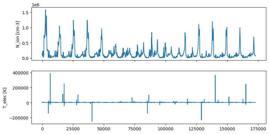

  []

  AppliedFilters :

  []

fig, (ax1, ax2) = plt.subplots(figsize=(10, 5), nrows=2, sharex=True)
def subplot(_ax, da):
    """Plot a given DataArray on a given axes"""
    _ax.plot(da)
    _ax.set_ylabel(f"{da.name} [{da.units}]")
for var, ax in zip(("N_ion", "T_elec"), (ax1, ax2)):
    subplot(ax, ds[var])