DNS (Thermospheric density)

%load_ext watermark
%watermark -i -v -p viresclient,pandas,xarray,matplotlib,cartopy

Python implementation: CPython
Python version       : 3.11.6
IPython version      : 8.18.0

viresclient: 0.15.0
pandas     : 2.1.3
xarray     : 2023.12.0
matplotlib : 3.8.2
cartopy    : 0.22.0

import datetime as dt

import matplotlib.pyplot as plt
import matplotlib as mpl
import pandas as pd
from viresclient import SwarmRequest

Product information

Thermospheric density products are available through the following collections, both from Swarm, and from other spacecraft (via the TOLEOS project)

• Thermospheric density derived from Swarm A, B, C (using the accelerometer):
  SW_OPER_DNSxACC_2_

• Thermospheric density derived from Swarm A, B, C (using only the orbit determination):
  SW_OPER_DNSxPOD_2_

• CHAMP:
  CH_OPER_DNS_ACC_2_

• GRACE 1 & 2:
  GR_OPER_DNSxACC_2_

• GRACE-FO 1:
  GF_OPER_DNSxACC_2_

We can check the available parameter names with:

request = SwarmRequest()
for collection in (
    "SW_OPER_DNSAACC_2_",
    "SW_OPER_DNSAPOD_2_",
    "CH_OPER_DNS_ACC_2_",
    "GR_OPER_DNS1ACC_2_",
    "GF_OPER_DNS1ACC_2_",
):
    print(f"{collection}:\n{request.available_measurements(collection)}\n")

SW_OPER_DNSAACC_2_:
['Height_GD', 'Latitude_GD', 'Longitude_GD', 'Height_GD', 'density', 'local_solar_time']

SW_OPER_DNSAPOD_2_:
['Height_GD', 'Latitude_GD', 'Longitude_GD', 'Height_GD', 'local_solar_time', 'density', 'density_orbitmean', 'validity_flag']

CH_OPER_DNS_ACC_2_:
['Height_GD', 'Latitude_GD', 'Longitude_GD', 'density', 'density_orbitmean', 'local_solar_time', 'validity_flag', 'validity_flag_orbitmean']

GR_OPER_DNS1ACC_2_:
['Height_GD', 'Latitude_GD', 'Longitude_GD', 'density', 'density_orbitmean', 'local_solar_time', 'validity_flag', 'validity_flag_orbitmean']

GF_OPER_DNS1ACC_2_:
['Height_GD', 'Latitude_GD', 'Longitude_GD', 'density', 'density_orbitmean', 'local_solar_time', 'validity_flag', 'validity_flag_orbitmean']

We can check for available time windows with:

request.available_times("SW_OPER_DNSAPOD_2_")

	starttime	endtime	bbox	identifier
0	2013-11-28 00:00:00+00:00	2013-11-28 23:59:30.001000+00:00	(-90,-180,90,180)	SW_OPER_DNSAPOD_2__20131128T000000_20131128T23...
1	2013-11-29 00:00:00+00:00	2013-11-29 23:59:30.001000+00:00	(-90,-180,90,180)	SW_OPER_DNSAPOD_2__20131129T000000_20131129T23...
2	2013-11-30 00:00:00+00:00	2013-11-30 23:59:30.001000+00:00	(-90,-180,90,180)	SW_OPER_DNSAPOD_2__20131130T000000_20131130T23...
3	2013-12-01 00:00:00+00:00	2013-12-01 23:59:30.001000+00:00	(-90,-180,90,180)	SW_OPER_DNSAPOD_2__20131201T000000_20131201T23...
4	2013-12-02 00:00:00+00:00	2013-12-02 23:59:30.001000+00:00	(-90,-180,90,180)	SW_OPER_DNSAPOD_2__20131202T000000_20131202T23...
...	...	...	...	...
4422	2026-01-27 00:00:00+00:00	2026-01-27 23:59:30.001000+00:00	(-90,-180,90,180)	SW_OPER_DNSAPOD_2__20260127T000000_20260127T23...
4423	2026-01-28 00:00:00+00:00	2026-01-28 23:59:30.001000+00:00	(-90,-180,90,180)	SW_OPER_DNSAPOD_2__20260128T000000_20260128T23...
4424	2026-01-29 00:00:00+00:00	2026-01-29 23:59:30.001000+00:00	(-90,-180,90,180)	SW_OPER_DNSAPOD_2__20260129T000000_20260129T23...
4425	2026-01-30 00:00:00+00:00	2026-01-30 23:59:30.001000+00:00	(-90,-180,90,180)	SW_OPER_DNSAPOD_2__20260130T000000_20260130T23...
4426	2026-01-31 00:00:00+00:00	2026-01-31 23:59:30.001000+00:00	(-90,-180,90,180)	SW_OPER_DNSAPOD_2__20260131T000000_20260131T23...

4427 rows × 4 columns

request.available_times("GF_OPER_DNS1ACC_2_")

	starttime	endtime	bbox	identifier
0	2018-05-29 00:00:00+00:00	2018-05-29 23:59:50.001000+00:00	(-90,-180,90,180)	GF_OPER_DNS1ACC_2__20180529T000000_20180529T23...
1	2018-05-30 00:00:00+00:00	2018-05-30 23:59:50.001000+00:00	(-90,-180,90,180)	GF_OPER_DNS1ACC_2__20180530T000000_20180530T23...
2	2018-05-31 00:00:00+00:00	2018-05-31 23:59:50.001000+00:00	(-90,-180,90,180)	GF_OPER_DNS1ACC_2__20180531T000000_20180531T23...
3	2018-06-01 00:00:00+00:00	2018-06-01 23:59:50.001000+00:00	(-90,-180,90,180)	GF_OPER_DNS1ACC_2__20180601T000000_20180601T23...
4	2018-06-02 00:00:00+00:00	2018-06-02 23:59:50.001000+00:00	(-90,-180,90,180)	GF_OPER_DNS1ACC_2__20180602T000000_20180602T23...
...	...	...	...	...
2762	2025-12-27 00:00:00+00:00	2025-12-27 23:59:50.001000+00:00	(-90,-180,90,180)	GF_OPER_DNS1ACC_2__20251227T000000_20251227T23...
2763	2025-12-28 00:00:00+00:00	2025-12-28 23:59:50.001000+00:00	(-90,-180,90,180)	GF_OPER_DNS1ACC_2__20251228T000000_20251228T23...
2764	2025-12-29 00:00:00+00:00	2025-12-29 23:59:50.001000+00:00	(-90,-180,90,180)	GF_OPER_DNS1ACC_2__20251229T000000_20251229T23...
2765	2025-12-30 00:00:00+00:00	2025-12-30 23:59:50.001000+00:00	(-90,-180,90,180)	GF_OPER_DNS1ACC_2__20251230T000000_20251230T23...
2766	2025-12-31 00:00:00+00:00	2025-12-31 23:59:50.001000+00:00	(-90,-180,90,180)	GF_OPER_DNS1ACC_2__20251231T000000_20251231T23...

2767 rows × 4 columns

Fetching neutral density

request = SwarmRequest()
request.set_collection(f"SW_OPER_DNSAACC_2_")
request.set_products(
    measurements=["density"],
)
data = request.get_between(dt.datetime(2015, 1, 1), dt.datetime(2015, 1, 2))
data.as_xarray()

<xarray.Dataset>
Dimensions:     (Timestamp: 8640)
Coordinates:
  * Timestamp   (Timestamp) datetime64[ns] 2015-01-01 ... 2015-01-01T23:59:50
Data variables:
    Spacecraft  (Timestamp) object 'A' 'A' 'A' 'A' 'A' ... 'A' 'A' 'A' 'A' 'A'
    Latitude    (Timestamp) float64 51.72 51.08 50.44 ... -72.17 -72.8 -73.43
    density     (Timestamp) float64 1.165e-12 1.174e-12 ... 9.99e+32 9.99e+32
    Radius      (Timestamp) float64 6.83e+06 6.83e+06 ... 6.844e+06 6.844e+06
    Longitude   (Timestamp) float64 -147.2 -147.1 -147.1 ... -136.5 -136.2
Attributes:
    Sources:         ['SW_OPER_DNSAACC_2__20150101T000000_20150101T235950_0201']
    MagneticModels:  []
    AppliedFilters:  []

xarray.Dataset

• Dimensions:
  • Timestamp: 8640
• Coordinates: (1)
  • Timestamp
    (Timestamp)
    datetime64[ns]
    2015-01-01 ... 2015-01-01T23:59:50

    description :

    array(['2015-01-01T00:00:00.000000000', '2015-01-01T00:00:10.000000000',
           '2015-01-01T00:00:20.000000000', ..., '2015-01-01T23:59:30.000000000',
           '2015-01-01T23:59:40.000000000', '2015-01-01T23:59:50.000000000'],
          dtype='datetime64[ns]')

• Data variables: (5)
  • Spacecraft
    (Timestamp)
    object
    'A' 'A' 'A' 'A' ... 'A' 'A' 'A' 'A'

    units :

    -

    description :

    Spacecraft identifier (values: 'A', 'B', 'C' or '-' if not available).

    array(['A', 'A', 'A', ..., 'A', 'A', 'A'], dtype=object)

  • Latitude
    (Timestamp)
    float64
    51.72 51.08 50.44 ... -72.8 -73.43

    units :

    deg

    description :

    Position in ITRF - Latitude

    array([ 51.71822133,  51.07910535,  50.43994905, ..., -72.17421626,
           -72.80457308, -73.4343609 ])

  • density
    (Timestamp)
    float64
    1.165e-12 1.174e-12 ... 9.99e+32

    units :

    kg/m3

    description :

    array([1.16484307e-12, 1.17404637e-12, 1.17793535e-12, ...,
           1.10074680e-12, 9.99000000e+32, 9.99000000e+32])

  • Radius
    (Timestamp)
    float64
    6.83e+06 6.83e+06 ... 6.844e+06

    units :

    m

    description :

    Position in ITRF - Radius

    array([6829956.61525865, 6830049.4417749 , 6830143.30951665, ...,
           6844317.14167012, 6844329.32496827, 6844341.14969496])

  • Longitude
    (Timestamp)
    float64
    -147.2 -147.1 ... -136.5 -136.2

    units :

    deg

    description :

    Position in ITRF - Longitude

    array([-147.15644399, -147.12218057, -147.08999172, ..., -136.74739106,
           -136.46355541, -136.15572558])

• Indexes: (1)
  • Timestamp
    PandasIndex

    PandasIndex(DatetimeIndex(['2015-01-01 00:00:00', '2015-01-01 00:00:10',
                   '2015-01-01 00:00:20', '2015-01-01 00:00:30',
                   '2015-01-01 00:00:40', '2015-01-01 00:00:50',
                   '2015-01-01 00:01:00', '2015-01-01 00:01:10',
                   '2015-01-01 00:01:20', '2015-01-01 00:01:30',
                   ...
                   '2015-01-01 23:58:20', '2015-01-01 23:58:30',
                   '2015-01-01 23:58:40', '2015-01-01 23:58:50',
                   '2015-01-01 23:59:00', '2015-01-01 23:59:10',
                   '2015-01-01 23:59:20', '2015-01-01 23:59:30',
                   '2015-01-01 23:59:40', '2015-01-01 23:59:50'],
                  dtype='datetime64[ns]', name='Timestamp', length=8640, freq=None))

• Attributes: (3)

  Sources :

  ['SW_OPER_DNSAACC_2__20150101T000000_20150101T235950_0201']

  MagneticModels :

  []

  AppliedFilters :

  []

Fetching from multiple spacecraft

We will fetch the data from around the geomagnetic storm event that affected a SpaceX Starlink launch and subsequent loss of spacecraft. See for example:
Starlink Satellite Losses During the February 2022 Geomagnetic Storm Event: Science, Technical and Economic Consequences, Policy, and Mitigation

def fetch_density(
    mission="SW", spacecraft="A", source="ACC", start_time=None, end_time=None
):
    request = SwarmRequest()
    request.set_collection(f"{mission}_OPER_DNS{spacecraft}{source}_2_")
    request.set_products(
        measurements=["density"],
        auxiliaries=["QDLat", "OrbitNumber", "OrbitDirection", "QDOrbitDirection"],
    )
    data = request.get_between(
        start_time, end_time, asynchronous=False, show_progress=False
    )
    return data.as_xarray()


start_time = dt.datetime(2022, 2, 1)
end_time = dt.datetime(2022, 2, 8)
# ds_SwA = fetch_density(mission="SW", spacecraft="A", source="POD", start_time=start_time, end_time=end_time)
# ds_SwB = fetch_density(mission="SW", spacecraft="B", source="POD", start_time=start_time, end_time=end_time)
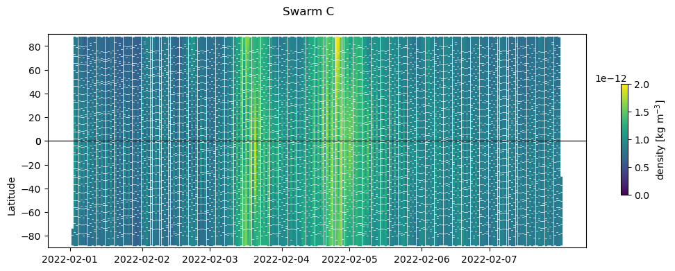
ds_SwC = fetch_density(
    mission="SW", spacecraft="C", source="POD", start_time=start_time, end_time=end_time
)
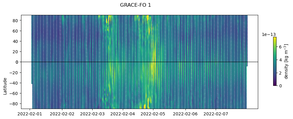
ds_GF1 = fetch_density(
    mission="GF", spacecraft="1", source="ACC", start_time=start_time, end_time=end_time
)

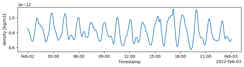
Now we have the data available from several datasets, e.g.:

# Use Swarm-C dataset, extract one day, and plot density
ds_SwC.sel(Timestamp=slice("2022-02-02", "2022-02-02"))["density"].plot.line(
    figsize=(10, 2)
);

You can check which source products have been accessed:

ds_SwC.attrs["Sources"]

['SW_OPER_AUXCORBCNT_20131122T132146_20260305T232403_0001',
 'SW_OPER_DNSCPOD_2__20220201T000000_20220201T235930_0301',
 'SW_OPER_DNSCPOD_2__20220202T000000_20220202T235930_0301',
 'SW_OPER_DNSCPOD_2__20220203T000000_20220203T235930_0301',
 'SW_OPER_DNSCPOD_2__20220204T000000_20220204T235930_0301',
 'SW_OPER_DNSCPOD_2__20220205T000000_20220205T235930_0301',
 'SW_OPER_DNSCPOD_2__20220206T000000_20220206T235930_0301',
 'SW_OPER_DNSCPOD_2__20220207T000000_20220207T235930_0301',
 'SW_OPER_MODC_SC_1B_20220131T000000_20220131T235959_0601',
 'SW_OPER_MODC_SC_1B_20220201T000000_20220201T235959_0601',
 'SW_OPER_MODC_SC_1B_20220202T000000_20220202T235959_0601',
 'SW_OPER_MODC_SC_1B_20220203T000000_20220203T235959_0601',
 'SW_OPER_MODC_SC_1B_20220204T000000_20220204T235959_0601',
 'SW_OPER_MODC_SC_1B_20220205T000000_20220205T235959_0601',
 'SW_OPER_MODC_SC_1B_20220206T000000_20220206T235959_0601',
 'SW_OPER_MODC_SC_1B_20220207T000000_20220207T235959_0601']

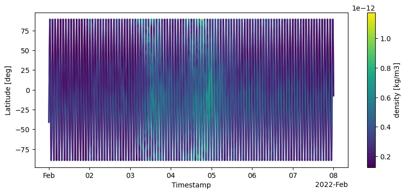
Visualisation example

Let’s try to display the density data as a function of time and latitude…

ds_GF1.plot.scatter(
    x="Timestamp", y="Latitude", hue="density", s=2, edgecolors="face", figsize=(10, 4)
);

Now let’s explore that a bit more to have more control over the figure

def select_north(ds):
    return ds.where(ds["Latitude"] > 0, drop=True)


def select_south(ds):
    return ds.where(ds["Latitude"] < 0, drop=True)


def select_ascending(ds):
    return ds.where(ds["OrbitDirection"] == 1, drop=True)


def select_descending(ds):
    return ds.where(ds["OrbitDirection"] == -1, drop=True)


def get_times_at_orbits(ds, orbitnos: list):
    da = ds["OrbitNumber"]
    t = []
    for orbitno in orbitnos:
        try:
            _t = (
                da.where(da == orbitno, drop=True)
                .isel({"Timestamp": 0})["Timestamp"]
                .values.astype("datetime64[s]")
                .astype(dt.datetime)
            )
        except IndexError:
            _t = None
        t.append(_t)
    return t


def get_orbits_at_times(ds, times: list):
    da = ds["OrbitNumber"]
    return list(da.sel(Timestamp=times, method="nearest").values.astype(int))

norm_gf = mpl.colors.Normalize(vmin=0, vmax=7.5e-13)
norm_sw = mpl.colors.Normalize(vmin=0, vmax=20e-13)


def plot_density(ds=ds_GF1, norm=norm_gf, title="GRACE-FO 1"):

    cmap = "viridis"
    plot_kwargs = {
        "norm": norm,
        "edgecolors": None,
        "s": 2,
        "marker": "s",
        "cmap": cmap,
    }

    fig, axes = plt.subplots(2, 1, figsize=(10, 4), sharex=True)
    # Plot the four segments of each orbit in sequence
    # North
    _ds = select_ascending(select_north(ds))
    axes[0].scatter(
        x=_ds["OrbitNumber"], y=_ds["Latitude"], c=_ds["density"], **plot_kwargs
    )
    _ds = select_descending(select_north(ds))
    axes[0].scatter(
        x=_ds["OrbitNumber"] + 0.5, y=_ds["Latitude"], c=_ds["density"], **plot_kwargs
    )
    # South
    _ds = select_descending(select_south(ds))
    axes[1].scatter(
        x=_ds["OrbitNumber"] + 0.5, y=_ds["Latitude"], c=_ds["density"], **plot_kwargs
    )
    _ds = select_ascending(select_south(ds))
    axes[1].scatter(
        x=_ds["OrbitNumber"] + 1.0, y=_ds["Latitude"], c=_ds["density"], **plot_kwargs
    )
    # Adjust axes
    axes[0].set_ylim(0, 90)
    axes[1].set_ylim(-90, 0)
    fig.subplots_adjust(hspace=0)
    axes[1].set_ylabel("Latitude")
    # axes[0].set_backgr
    fig.suptitle(title)
    # Move xticks to align with day starts
    t_start_end = (
        ds["Timestamp"]
        .isel(Timestamp=[0, -1])
        .values.astype("datetime64[s]")
        .astype(dt.datetime)
    )
    times_to_mark = pd.date_range(start=t_start_end[0], end=t_start_end[1], freq="D")
    orbits_to_mark = get_orbits_at_times(ds, times_to_mark)
    axes[1].set_xticks(orbits_to_mark)
    # Replace orbit numbers with the times
    times_formatted = [_t.strftime("%Y-%m-%d") for _t in times_to_mark]
    axes[1].set_xticklabels(times_formatted)
    # Add colorbar
    cbar_ax = fig.add_axes([0.95, 0.3, 0.01, 0.4])
    sm = mpl.cm.ScalarMappable(cmap=plot_kwargs["cmap"], norm=plot_kwargs["norm"])
    sm.set_array([])
    cb = fig.colorbar(sm, cax=cbar_ax)
    cb.set_label("density [kg m$^{-3}$]")

plot_density(ds_GF1, norm_gf, "GRACE-FO 1")

plot_density(ds_SwC, norm_sw, "Swarm C")