FACxTMS_2F (single spacecraft)

FACxTMS_2F (single spacecraft)#

Abstract: Access to the field aligned currents evaluated by the single satellite method (level 2 product). We show simple line plots of the time series over short periods (minutes), from both Swarm Alpha and Charlie. We also compare with the alternative method whereby the FACs are evaluated locally by computing them from the magnetic field data (B_NEC from MAGx_LR_1B).

%load_ext watermark
%watermark -i -v -p viresclient,pandas,xarray,matplotlib

Python implementation: CPython
Python version       : 3.11.6
IPython version      : 8.18.0

viresclient: 0.15.0
pandas     : 2.1.3
xarray     : 2023.12.0
matplotlib : 3.8.2

Product information#

Documentation:

from viresclient import SwarmRequest
import datetime as dt
import numpy as np
import pandas as pd
import matplotlib.pyplot as plt
import matplotlib.dates as mdates
import cartopy.crs as ccrs
import cartopy.feature as cfeature

request = SwarmRequest()

Check what “FAC” data variables are available#

NB: these are the same as in the FAC_TMS_2F dual-satellite FAC product

request.available_collections("FAC", details=False)

{'FAC': ['SW_OPER_FACATMS_2F',
  'SW_OPER_FACBTMS_2F',
  'SW_OPER_FACCTMS_2F',
  'SW_OPER_FAC_TMS_2F',
  'SW_FAST_FACATMS_2F',
  'SW_FAST_FACBTMS_2F',
  'SW_FAST_FACCTMS_2F']}

request.available_measurements("FAC")

['IRC',
 'IRC_Error',
 'FAC',
 'FAC_Error',
 'Flags',
 'Flags_F',
 'Flags_B',
 'Flags_q']

Plotting as a time series#

Fetch one day from Swarm Alpha and Charlie#

Also fetch the quasidipole (QD) coordinates and Orbit Number at the same time.

request.set_collection("SW_OPER_FACATMS_2F", "SW_OPER_FACCTMS_2F")
request.set_products(
    measurements=["FAC", "FAC_Error", "Flags", "Flags_F", "Flags_B", "Flags_q"],
    auxiliaries=["QDLat", "QDLon", "OrbitNumber"],
)
data = request.get_between(dt.datetime(2014, 4, 20), dt.datetime(2014, 4, 21))

The source files of the original data are listed

data.sources

['SW_OPER_AUXAORBCNT_20131122T132146_20260305T232412_0001',
 'SW_OPER_AUXCORBCNT_20131122T132146_20260305T232403_0001',
 'SW_OPER_FACATMS_2F_20140420T000000_20140420T235959_0401',
 'SW_OPER_FACCTMS_2F_20140420T000000_20140420T235959_0401']

The data can be loaded as a pandas dataframe

df = data.as_dataframe()
df = df.sort_index()
df.head()

	QDLon	FAC_Error	Spacecraft	Longitude	Flags_q	Radius	Latitude	Flags_B	FAC	OrbitNumber	Flags	Flags_F	QDLat
Timestamp
2014-04-20 00:00:00.500	87.677834	0.065509	A	19.102806	0	6851356.835	-26.849185	0	0.004292	2267	0	2	-36.222500
2014-04-20 00:00:00.500	89.366638	0.062153	C	20.535146	0	6851317.060	-26.285007	0	-0.020003	2263	0	2	-35.770004
2014-04-20 00:00:01.500	89.390350	0.065763	C	20.534623	0	6851310.440	-26.221325	0	0.003943	2263	0	2	-35.718651
2014-04-20 00:00:01.500	87.701981	0.065887	A	19.102319	0	6851350.325	-26.785506	0	0.006710	2267	0	2	-36.172028
2014-04-20 00:00:02.500	87.726082	0.066541	A	19.101828	0	6851343.805	-26.721826	0	0.010963	2267	0	2	-36.121506

Alternatively we can load the data as an xarray Dataset, though in the following examples we use the data via a pandas DataFrame instead

Depending on your application, you should probably do some filtering according to each of the flags. This can be done on the dataframe here, or beforehand on the server using request.set_range_filter(). See https://earth.esa.int/documents/10174/1514862/Swarm_L2_FAC_single_product_description for more about the data

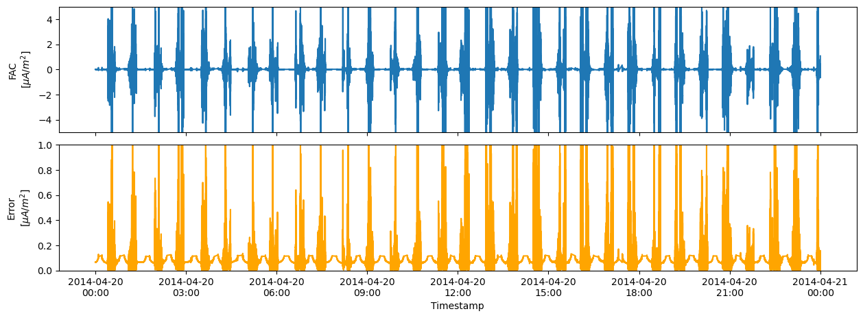
Plot the time series (FAC and FAC_Error for Alpha)#

fig, axes = plt.subplots(ncols=1, nrows=2, figsize=(15, 5))
# Select out the time series from Swarm Alpha
dfA = df.where(df["Spacecraft"] == "A").dropna()
axes[0].plot(dfA.index, dfA["FAC"])
axes[1].plot(dfA.index, dfA["FAC_Error"], color="orange")
axes[0].set_ylabel("FAC\n[$\mu A / m^2$]")
axes[1].set_ylabel("Error\n[$\mu A / m^2$]")
axes[1].set_xlabel("Timestamp")
date_format = mdates.DateFormatter("%Y-%m-%d\n%H:%M")
axes[1].xaxis.set_major_formatter(date_format)
axes[0].set_ylim(-5, 5)
axes[1].set_ylim(0, 1)
axes[0].set_xticklabels([])
fig.subplots_adjust(hspace=0.1)

../_images/7820f949aa8c467543a4bdf71a4271d7b2c04cc077302ea20d82a8930ad47cab.png

Plot a subset of the time series (FAC from Alpha and Charlie)#

def line_plot(fig, ax, df, varname="FAC", spacecraft="A", color="red"):
    """Plot FAC as a line, given a dataframe"""
    df = df.copy()
    df = df.where(df["Spacecraft"] == spacecraft).dropna()
    ax.plot(
        df.index,
        df[varname],
        linewidth=1,
        label=f"{varname}$_{spacecraft}$",
        color=color,
    )
    # Plot error range as filled area
    if varname == "FAC":
        ax.fill_between(
            df.index,
            df["FAC"] - df["FAC_Error"],
            df["FAC"] + df["FAC_Error"],
            color="grey",
        )
    # Adjust limits and label formatting
    datetime_format = "%Y-%m-%d\n%H:%M:%S"
    xlabel_format = mdates.DateFormatter(datetime_format)
    ax.xaxis.set_major_formatter(xlabel_format)
    ax.set_ylabel("[ $\mu A / m^2$ ]")
    # Make y-axis symmetric about zero
    ylim = max(abs(y) for y in ax.get_ylim())
    ax.set_ylim((-ylim, ylim))
    ax.legend()
    ax.grid(True)
    # Set up an extra xaxis at the top, to display Latitude
    ax2 = ax.twiny()
    ax2.set_xlim(ax.get_xlim())
    ax2.set_xticks(ax.get_xticks())
    # Identify closest times in dataframe to use for Latitude labels
    # NB need to draw the figure now in order to get the xticklabels
    #  https://stackoverflow.com/a/41124884
    fig.canvas.draw()
    # Extract times from the lower x axis
    # Use them to find the nearest Lat values in the dataframe
    xtick_times = [
        dt.datetime.strptime(ts.get_text(), datetime_format)
        for ts in ax.get_xticklabels()
    ]
    ilocs = [df.index.get_indexer([t], method="nearest")[0] for t in xtick_times]
    lats = df.iloc[ilocs]["Latitude"]
    lat_labels = ["{}°".format(s) for s in np.round(lats.values, decimals=1)]
    ax2.set_xticklabels(lat_labels)
    ax2.set_xlabel("Latitude")


# Easy pandas-style slicing of the dataframe
df_subset = df["2014-04-20T04:26:00":"2014-04-20T04:30:00"]
fig, axes = plt.subplots(nrows=2, figsize=(15, 5))
line_plot(fig, axes[0], df_subset, spacecraft="A", color="red")
line_plot(fig, axes[1], df_subset, spacecraft="C", color="blue")
fig.subplots_adjust(hspace=0.8)

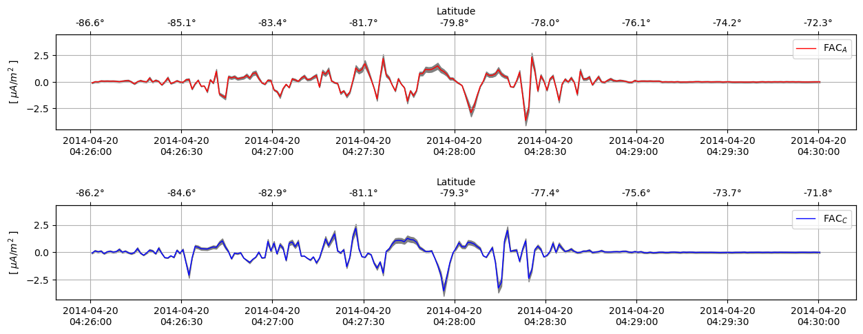
../_images/42150d146db53b2a1cec38fef720b018fadb1ce612d2a68ba5814624d5dcb01f.png

FAC estimates from (top) Swarm Alpha and (bottom) Swarm Charlie. The error estimate is shown as a thin grey area

Also show satellite location on a map#

def line_plot_figure(df, spacecraft="A", color="red"):
    """Generate a figure containing both line plot and maps"""
    df = df.copy()
    df = df.where(df["Spacecraft"] == spacecraft).dropna()
    # Set up figure geometry together with North/South maps
    fig = plt.figure(figsize=(20, 5))
    ax_lineplot = plt.subplot2grid((1, 5), (0, 0), colspan=3, fig=fig)
    ax_N = plt.subplot2grid(
        (1, 5),
        (0, 3),
        fig=fig,
        projection=ccrs.Orthographic(central_longitude=0.0, central_latitude=90.0),
    )
    ax_S = plt.subplot2grid(
        (1, 5),
        (0, 4),
        fig=fig,
        projection=ccrs.Orthographic(central_longitude=0.0, central_latitude=-90.0),
    )
    for _ax in (ax_N, ax_S):
        _ax.set_global()
        _ax.coastlines(color="grey")
        _ax.add_feature(cfeature.LAND)
        _ax.add_feature(cfeature.OCEAN)
        _ax.plot(
            df["Longitude"],
            df["Latitude"],
            transform=ccrs.PlateCarree(),
            linewidth=4,
            color=color,
        )
    # Draw the line plot as before
    line_plot(fig, ax_lineplot, df, spacecraft=spacecraft, color=color)


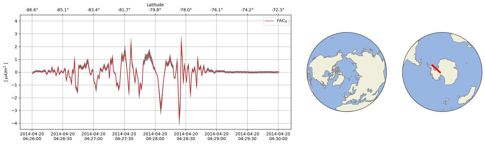
line_plot_figure(df_subset, spacecraft="A", color="red")

/opt/conda/lib/python3.11/site-packages/cartopy/io/__init__.py:241: DownloadWarning: Downloading: https://naturalearth.s3.amazonaws.com/110m_physical/ne_110m_land.zip
  warnings.warn(f'Downloading: {url}', DownloadWarning)

/opt/conda/lib/python3.11/site-packages/cartopy/io/__init__.py:241: DownloadWarning: Downloading: https://naturalearth.s3.amazonaws.com/110m_physical/ne_110m_ocean.zip
  warnings.warn(f'Downloading: {url}', DownloadWarning)

/opt/conda/lib/python3.11/site-packages/cartopy/io/__init__.py:241: DownloadWarning: Downloading: https://naturalearth.s3.amazonaws.com/110m_physical/ne_110m_coastline.zip
  warnings.warn(f'Downloading: {url}', DownloadWarning)

../_images/e1f275b93a0ccbe143053b9bf75fd6e7fc04505da6e331f737085f5f43697b23.png