IPDxIRR_2F (Ionospheric plasma densities)#
Abstract: Access to the derived plasma characteristics at 1Hz (level 2 product).
%load_ext watermark
%watermark -i -v -p viresclient,pandas,xarray,matplotlib
Python implementation: CPython
Python version       : 3.11.6
IPython version      : 8.18.0

viresclient: 0.15.0
pandas     : 2.1.3
xarray     : 2023.12.0
matplotlib : 3.8.2
from viresclient import SwarmRequest
import datetime as dt
import matplotlib.pyplot as plt
from matplotlib.dates import DateFormatter

request = SwarmRequest()
IPDxIRR_2F product information#
Derived plasma characteristics at 1Hz, for each Swarm spacecraft.
Documentation:
Check what “IPD” data variables are available#
request.available_collections("IPD", details=False)
{'IPD': ['SW_OPER_IPDAIRR_2F', 'SW_OPER_IPDBIRR_2F', 'SW_OPER_IPDCIRR_2F']}
request.available_measurements("IPD")
['Ne',
 'Te',
 'Background_Ne',
 'Foreground_Ne',
 'PCP_flag',
 'Grad_Ne_at_100km',
 'Grad_Ne_at_50km',
 'Grad_Ne_at_20km',
 'Grad_Ne_at_PCP_edge',
 'ROD',
 'RODI10s',
 'RODI20s',
 'delta_Ne10s',
 'delta_Ne20s',
 'delta_Ne40s',
 'Num_GPS_satellites',
 'mVTEC',
 'mROT',
 'mROTI10s',
 'mROTI20s',
 'IBI_flag',
 'Ionosphere_region_flag',
 'IPIR_index',
 'Ne_quality_flag',
 'TEC_STD']
Fetch three hours of IPD data#
request.set_collection("SW_OPER_IPDAIRR_2F")
request.set_products(measurements=request.available_measurements("IPD"))
data = request.get_between(dt.datetime(2014, 12, 21, 0), dt.datetime(2014, 12, 21, 3))
Load and plot using pandas/matplotlib#
df = data.as_dataframe()
df.head()
| Num_GPS_satellites | Longitude | ROD | IPIR_index | Grad_Ne_at_100km | delta_Ne10s | mROTI10s | Ne | Te | Spacecraft | ... | Grad_Ne_at_20km | TEC_STD | Latitude | Radius | Ne_quality_flag | mVTEC | mROTI20s | delta_Ne20s | Ionosphere_region_flag | Background_Ne | |
|---|---|---|---|---|---|---|---|---|---|---|---|---|---|---|---|---|---|---|---|---|---|
| Timestamp | |||||||||||||||||||||
| 2014-12-21 00:00:00.196999936 | 4 | -128.771412 | 0.0 | 7 | -0.084919 | 67.875 | 0.001472 | 1255163.2 | 2212.278353 | A | ... | -1.047788 | 3.131451 | -4.693533 | 6.840395e+06 | 20000 | 51.786934 | 0.002676 | 10266.500 | 0 | 1343599.375 |
| 2014-12-21 00:00:01.196999936 | 4 | -128.772618 | 0.0 | 6 | -0.144009 | 12961.600 | 0.001386 | 1250357.7 | 2165.194729 | A | ... | 0.338403 | 3.122494 | -4.757416 | 6.840404e+06 | 20000 | 51.768982 | 0.002732 | 2830.850 | 0 | 1343599.375 |
| 2014-12-21 00:00:02.196999936 | 4 | -128.773822 | 0.0 | 6 | -0.058276 | 0.000 | 0.001310 | 1265851.3 | 1544.874194 | A | ... | 0.133643 | 3.113830 | -4.821298 | 6.840413e+06 | 20000 | 51.746898 | 0.002750 | 0.000 | 0 | 1343599.375 |
| 2014-12-21 00:00:03.196999936 | 4 | -128.775026 | 0.0 | 6 | -0.144613 | 12393.550 | 0.001930 | 1312436.8 | 1228.501871 | A | ... | 1.443077 | 3.104259 | -4.885179 | 6.840422e+06 | 20000 | 51.728759 | 0.003277 | 2194.925 | 0 | 1343599.375 |
| 2014-12-21 00:00:04.196999936 | 4 | -128.776229 | 0.0 | 6 | -0.039358 | 21700.700 | 0.002434 | 1253999.0 | 2681.512355 | A | ... | -1.948789 | 3.097484 | -4.949060 | 6.840430e+06 | 20000 | 51.711313 | 0.003744 | 9491.525 | 0 | 1343599.375 |
5 rows × 29 columns
df.columns
Index(['Num_GPS_satellites', 'Longitude', 'ROD', 'IPIR_index',
       'Grad_Ne_at_100km', 'delta_Ne10s', 'mROTI10s', 'Ne', 'Te', 'Spacecraft',
       'IBI_flag', 'Foreground_Ne', 'Grad_Ne_at_50km', 'Grad_Ne_at_PCP_edge',
       'PCP_flag', 'RODI10s', 'RODI20s', 'delta_Ne40s', 'mROT',
       'Grad_Ne_at_20km', 'TEC_STD', 'Latitude', 'Radius', 'Ne_quality_flag',
       'mVTEC', 'mROTI20s', 'delta_Ne20s', 'Ionosphere_region_flag',
       'Background_Ne'],
      dtype='object')
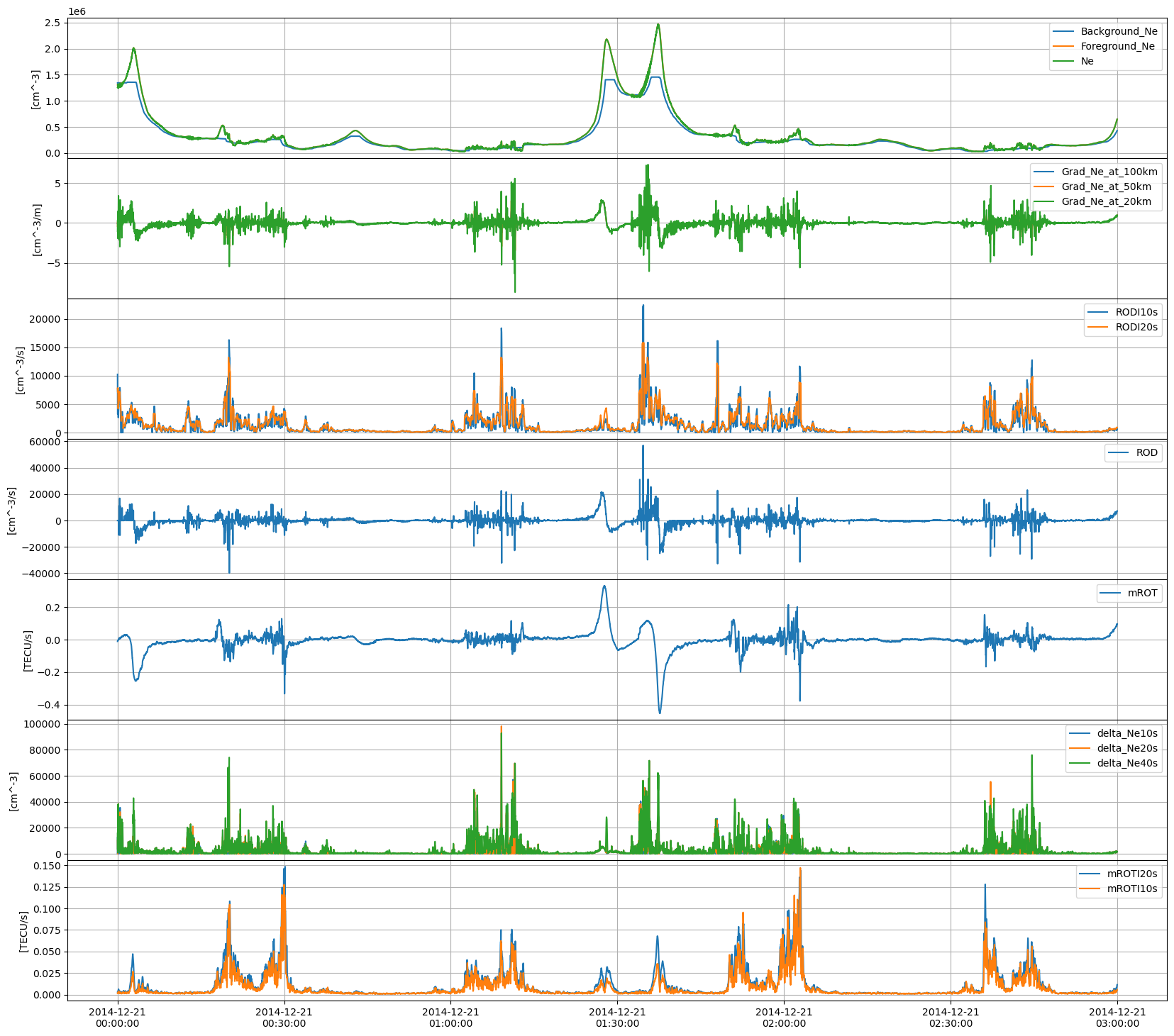
fig, axes = plt.subplots(nrows=7, ncols=1, figsize=(20, 18), sharex=True)
df.plot(ax=axes[0], y=["Background_Ne", "Foreground_Ne", "Ne"], alpha=0.8)
df.plot(ax=axes[1], y=["Grad_Ne_at_100km", "Grad_Ne_at_50km", "Grad_Ne_at_20km"])
df.plot(ax=axes[2], y=["RODI10s", "RODI20s"])
df.plot(ax=axes[3], y=["ROD"])
df.plot(ax=axes[4], y=["mROT"])
df.plot(ax=axes[5], y=["delta_Ne10s", "delta_Ne20s", "delta_Ne40s"])
df.plot(ax=axes[6], y=["mROTI20s", "mROTI10s"])
axes[0].set_ylabel("[cm$^{-3}$]")
axes[1].set_ylabel("[cm$^{-3}$m$^{-1}$]")
axes[2].set_ylabel("[cm$^{-3}$s$^{-1}$]")
axes[3].set_ylabel("[cm$^{-3}$m$^{-1}$]")
axes[4].set_ylabel("[TECU s$^{-1}$]")
axes[5].set_ylabel("[cm$^{-3}$m$^{-1}$]")
axes[6].set_ylabel("[TECU s$^{-1}$]")
axes[6].set_xlabel("Timestamp")

for ax in axes:
    # Reformat time axis
    # https://www.earthdatascience.org/courses/earth-analytics-python/use-time-series-data-in-python/customize-dates--matplotlib-plots-python/
    ax.xaxis.set_major_formatter(DateFormatter("%Y-%m-%d\n%H:%M:%S"))
    ax.legend(loc="upper right")
    ax.grid()
fig.subplots_adjust(hspace=0)
Load as xarray#
ds = data.as_xarray()
ds
<xarray.Dataset>
Dimensions:                 (Timestamp: 10800)
Coordinates:
  * Timestamp               (Timestamp) datetime64[ns] 2014-12-21T00:00:00.19...
Data variables: (12/29)
    Spacecraft              (Timestamp) object 'A' 'A' 'A' 'A' ... 'A' 'A' 'A'
    Num_GPS_satellites      (Timestamp) int32 4 4 4 4 4 4 4 4 ... 6 6 6 6 6 6 6
    Longitude               (Timestamp) float64 -128.8 -128.8 ... -175.4 -175.4
    ROD                     (Timestamp) float64 0.0 0.0 ... 7.28e+03 7.28e+03
    IPIR_index              (Timestamp) int32 7 6 6 6 6 6 6 6 ... 4 4 4 4 4 4 4
    Grad_Ne_at_100km        (Timestamp) float64 -0.08492 -0.144 ... 0.9621
    ...                      ...
    Ne_quality_flag         (Timestamp) int32 20000 20000 20000 ... 10000 10000
    mVTEC                   (Timestamp) float64 51.79 51.77 ... 20.84 20.94
    mROTI20s                (Timestamp) float64 0.002676 0.002732 ... 0.0114
    delta_Ne20s             (Timestamp) float64 1.027e+04 ... 1.702e+03
    Ionosphere_region_flag  (Timestamp) int32 0 0 0 0 0 0 0 0 ... 0 0 0 0 0 0 0
    Background_Ne           (Timestamp) float64 1.344e+06 1.344e+06 ... 4.29e+05
Attributes:
    Sources:         ['SW_OPER_IPDAIRR_2F_20141221T000000_20141221T235959_0302']
    MagneticModels:  []
AppliedFilters: []Alternative plot setup#
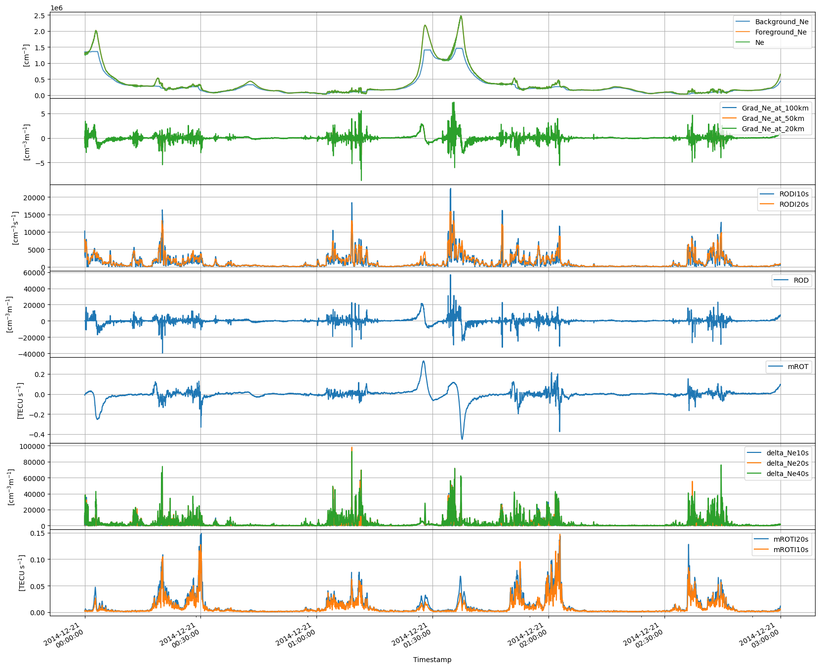
To plot the data from xarray, we need a different plotting setup. This does however give us more control over the plot. The units are extracted directly from the xarray object.
fig, axes = plt.subplots(nrows=7, ncols=1, figsize=(20, 18), sharex=True)


def subplot(ax=None, y=None, **kwargs):
    """Plot combination of variables onto a given axis"""
    units = ds[y[0]].units
    for var in y:
        ax.plot(ds["Timestamp"], ds[var], label=var, **kwargs)
        if units != ds[var].units:
            raise ValueError(f"Units mismatch for {var}")
    ax.set_ylabel(f"[{units}]")
    # Reformat time axis
    # https://www.earthdatascience.org/courses/earth-analytics-python/use-time-series-data-in-python/customize-dates--matplotlib-plots-python/
    ax.xaxis.set_major_formatter(DateFormatter("%Y-%m-%d\n%H:%M:%S"))
    ax.legend(loc="upper right")
    ax.grid()


subplot(ax=axes[0], y=["Background_Ne", "Foreground_Ne", "Ne"])
subplot(ax=axes[1], y=["Grad_Ne_at_100km", "Grad_Ne_at_50km", "Grad_Ne_at_20km"])
subplot(ax=axes[2], y=["RODI10s", "RODI20s"])
subplot(ax=axes[3], y=["ROD"])
subplot(ax=axes[4], y=["mROT"])
subplot(ax=axes[5], y=["delta_Ne10s", "delta_Ne20s", "delta_Ne40s"])
subplot(ax=axes[6], y=["mROTI20s", "mROTI10s"])
fig.subplots_adjust(hspace=0)