IBP-Model#
Notebook authors: Ina Rusch
Package authors: Martin Rother, Ina Rusch
Resources#
Python package: ibpmodel
Code
Documentation
Swarm Data Handbook
Basic usage#
import ibpmodel as ibp
import numpy as np
import matplotlib.pyplot as plt
Calculate the IBP model at given time of year, position, and conditions:
ibp.calculateIBPindex(
    day_month=15,  # Day of Year or Month
    longitude=0,  # Longitude in degree
    local_time=20.9,  # Local time in hours
    f107=150,  # F10.7 cm Solar Flux index
)
| Doy | Month | Lon | LT | F10.7 | IBP | |
|---|---|---|---|---|---|---|
| 0 | 15 | 1 | 0 | 20.9 | 150 | 0.3433 |
ibp.calculateIBPindex(day_month=["Jan", "Feb", "Mar"], local_time=22)
| Doy | Month | Lon | LT | F10.7 | IBP | |
|---|---|---|---|---|---|---|
| 0 | 15 | 1 | -180 | 22 | 150 | 0.0655 |
| 1 | 15 | 1 | -175 | 22 | 150 | 0.0667 |
| 2 | 15 | 1 | -170 | 22 | 150 | 0.0685 |
| 3 | 15 | 1 | -165 | 22 | 150 | 0.0710 |
| 4 | 15 | 1 | -160 | 22 | 150 | 0.0754 |
| ... | ... | ... | ... | ... | ... | ... |
| 211 | 74 | 3 | 155 | 22 | 150 | 0.2146 |
| 212 | 74 | 3 | 160 | 22 | 150 | 0.2123 |
| 213 | 74 | 3 | 165 | 22 | 150 | 0.2117 |
| 214 | 74 | 3 | 170 | 22 | 150 | 0.2119 |
| 215 | 74 | 3 | 175 | 22 | 150 | 0.2123 |
216 rows × 6 columns
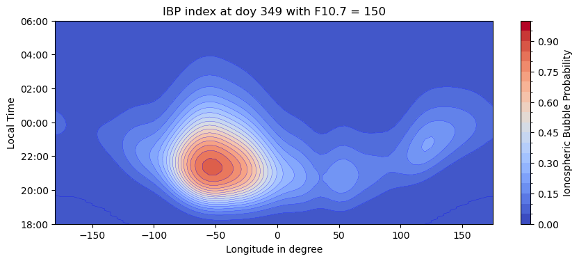
Plot the global pattern for a given day:
ibp.plotIBPindex(doy=349)
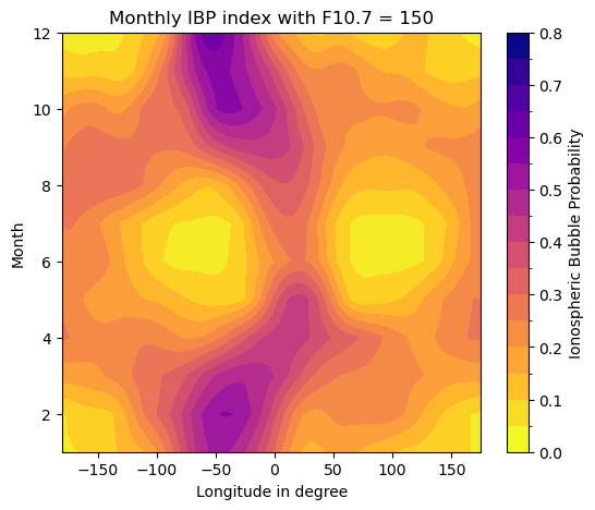
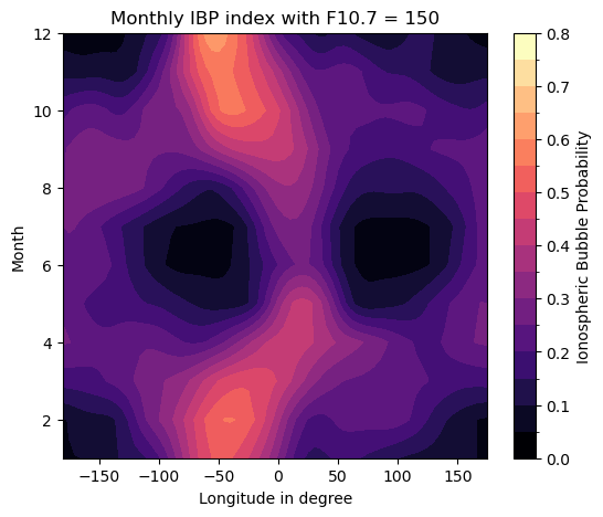
Plot the month vs longitude pattern:
ibp.plotButterflyData(f107=150)
More examples#
ibp.calculateIBPindex("Jan", longitude=170, local_time=np.arange(-2, -1, 0.1))
| Doy | Month | Lon | LT | F10.7 | IBP | |
|---|---|---|---|---|---|---|
| 0 | 15 | 1 | 170 | -2.0 | 150 | 0.0682 |
| 1 | 15 | 1 | 170 | -1.9 | 150 | 0.0727 |
| 2 | 15 | 1 | 170 | -1.8 | 150 | 0.0769 |
| 3 | 15 | 1 | 170 | -1.7 | 150 | 0.0808 |
| 4 | 15 | 1 | 170 | -1.6 | 150 | 0.0842 |
| 5 | 15 | 1 | 170 | -1.5 | 150 | 0.0872 |
| 6 | 15 | 1 | 170 | -1.4 | 150 | 0.0897 |
| 7 | 15 | 1 | 170 | -1.3 | 150 | 0.0917 |
| 8 | 15 | 1 | 170 | -1.2 | 150 | 0.0931 |
| 9 | 15 | 1 | 170 | -1.1 | 150 | 0.0940 |
ibp.calculateIBPindex(
    day_month=[1, 15, 31], longitude=[-170, 175, 170], local_time=0, f107=150
)
| Doy | Month | Lon | LT | F10.7 | IBP | |
|---|---|---|---|---|---|---|
| 0 | 1 | 1 | -170 | 0 | 150 | 0.0735 |
| 1 | 1 | 1 | 175 | 0 | 150 | 0.0704 |
| 2 | 1 | 1 | 170 | 0 | 150 | 0.0714 |
| 3 | 15 | 1 | -170 | 0 | 150 | 0.0773 |
| 4 | 15 | 1 | 175 | 0 | 150 | 0.0740 |
| 5 | 15 | 1 | 170 | 0 | 150 | 0.0751 |
| 6 | 31 | 1 | -170 | 0 | 150 | 0.0868 |
| 7 | 31 | 1 | 175 | 0 | 150 | 0.0831 |
| 8 | 31 | 1 | 170 | 0 | 150 | 0.0843 |
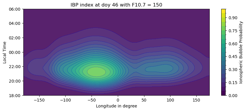
ibp.plotIBPindex("Feb", cmap="viridis", alpha=0.9)
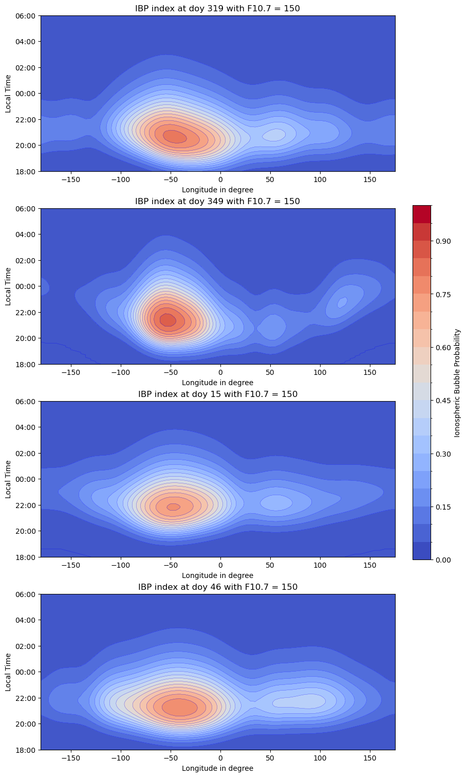
doys = [319, 349, 15, 46]
fig_doys, axes_doys = plt.subplots(len(doys), 1, layout="constrained", figsize=(9, 15))

for d, ax in zip(doys, axes_doys):
    ax, scalarmap = ibp.plotIBPindex(d, ax=ax)

ibp.ibpforward.setcolorbar(scalarmap, fig_doys, axes_doys, fraction=0.05)
plt.show()
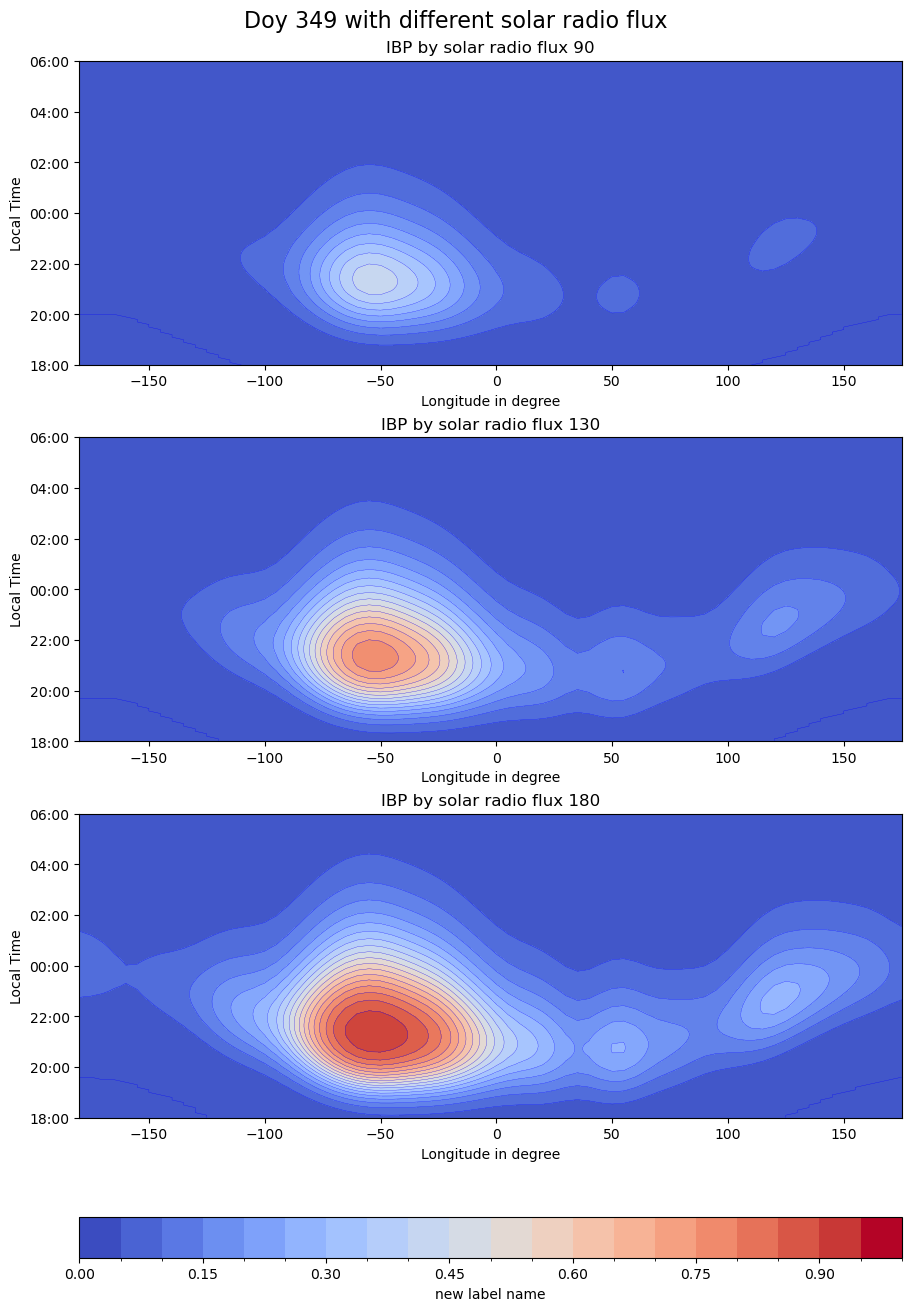
solar = [90, 130, 180]
doy = 349
fig_solar, axes_solar = plt.subplots(
    len(solar), 1, layout="constrained", figsize=(9, 13)
)
fig_solar.suptitle(f"Doy {doy} with different solar radio flux", fontsize=16)

for f, ax in zip(solar, axes_solar):
    ax, scalarmap = ibp.plotIBPindex(doy, f107=f, ax=ax)
    ax.set_title(f"IBP by solar radio flux {f}")

cbar = ibp.ibpforward.setcolorbar(
    scalarmap, fig_solar, axes_solar, fraction=0.05, orientation="horizontal"
)
cbar.set_label("new label name")
ibp.plotButterflyData(150, cmap="magma")
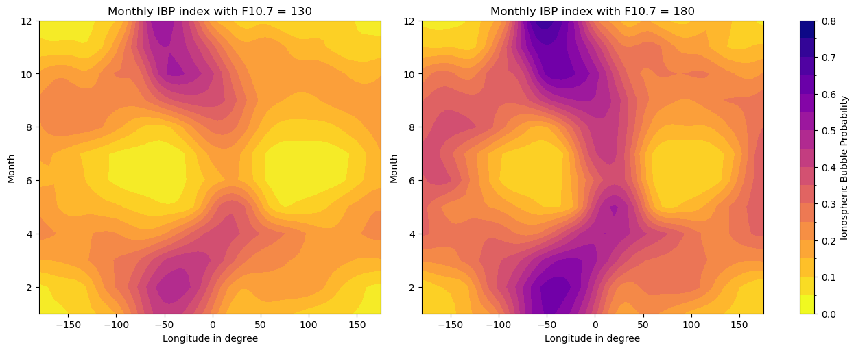
solar = [130, 180]
fig_bfly, axes_bfly = plt.subplots(
    1, len(solar), layout="constrained", figsize=(12.4, 5)
)

for b, ax in zip(solar, axes_bfly):
    ax, scalarmap = ibp.plotButterflyData(b, ax=ax)

ibp.ibpforward.setcolorbar(scalarmap, fig_bfly, axes_bfly)
plt.show()
Visualisation along Swarm orbits#
Source:
https://igit.iap-kborn.de/ibp/ibp-model/-/blob/main/template/IBP-VirES.ipynb
%pip install --quiet lxml
WARNING: Running pip as the 'root' user can result in broken permissions and conflicting behaviour with the system package manager, possibly rendering your system unusable. It is recommended to use a virtual environment instead: https://pip.pypa.io/warnings/venv. Use the --root-user-action option if you know what you are doing and want to suppress this warning.
Note: you may need to restart the kernel to use updated packages.
import ibpmodel as ibp
import numpy as np
import pandas as pd
import matplotlib.pyplot as plt
from datetime import datetime, timezone, timedelta, date
from viresclient import SwarmRequest
def getlt(datum, lon):
    """Output of the day of the year and local time for specifying date(s) and longitude(s).

    Parameters
    ----------
    datum : datetime or list of datetimes
    lon : int or list of int
        The geographical longitude, ``-180 <= longitude <= 180``.

    Returns
    -------
    tupel
        contains (list of) day(s) of the year and (list of) local time(s)
    """

    def calclt(date, lon):
        return round(
            (date.hour + date.minute / 60 + date.second / 3600 + 24 * lon / 360) % 24, 1
        )

    if isinstance(datum, datetime):
        doys = int(datum.strftime("%j"))
        lts = calclt(datum, lon)

    elif isinstance(datum, list):
        doys = []
        lts = []
        for d, l in zip(datum, lon):
            doys.append(int(d.strftime("%j")))
            lts.append(calclt(d, l))

    return (doys, lts)


def loadsatellitedata(starttime, endtime, satellite):
    """Load data via viresclient

    Parameters
    ----------
    starttime : datetime
    endtime : datetime
    satellite : str
        name of satellite

    Returns
    -------
    pandas.DataFrame

    """
    request = SwarmRequest()
    request.set_collection(f"SW_OPER_IBI{satellite}TMS_2F")
    request.set_products(
        measurements=request.available_measurements("IBI"),
        auxiliaries=["F10_INDEX", "F107"],
    )
    data = request.get_between(starttime, endtime)
    df = data.as_dataframe()
    df = df[(df.Bubble_Index > -1)]

    return df


def downloadfn(dates):
    """Download Solar Radio Flux for specified date(s).

    Parameters
    ----------
    dates : datetime or list of datetimes

    Returns
    -------
    list of numpy.float64
        Solar Radio Flux
    """

    def loaddf(year):
        df = pd.read_html(
            f"https://spaceweather.gc.ca/forecast-prevision/solar-solaire/solarflux/sx-5-flux-en.php?year={year}"
        )[0]
        return df

    def getfn(df, date):
        return df[(df.Date == date.strftime("%Y-%m-%d")) & (df.Time == "20:00:00")][
            "Observed Flux"
        ].values[0]

    if isinstance(dates, datetime):
        years = [dates.year]
        dates = [dates]
    elif isinstance(dates, list):
        years = [dates[0].year]
    else:
        raise TypeError(f"must be datetime or list of datetimes")

    df_fn = loaddf(years[0])
    fn = []

    for d in dates:
        y = d.year
        if y not in years:
            df_fn = pd.concat([df_fn, loaddf(y)])
            fn.append(getfn(df_fn, d))
            years.append(y)
        else:
            fn.append(getfn(df_fn, d))

    return fn


def calcindex(df):
    """Calculation of the IBP index. If Solar Radio Flux lower than 80 the IBP index is set to -1.

    Parameters
    ----------
    df : pandas.DataFrame (with columns Doy, Lon, LT and F10.7)

    Returns
    -------
    pandas.DataFrame
        contains the columns: Doy (Day(s) of the year), Month (Month(s) from the day of the year),
        Lon (Longitude(s)), LT (Local Time(s)), F10.7 (solar index(es)), IBP (Ionospheric Bubble Index, value(s) between 0.0 and 1.0).
    """

    def calcibp(index, row):
        df = ibp.calculateIBPindex(
            day_month=int(row["Doy"]),
            longitude=row["Lon"],
            local_time=row["LT"],
            f107=row["F10.7"],
        )
        df = df.set_index([pd.Index([index])])
        return df

    index_sort = df.index

    tmp = df[(df["F10.7"] < 80)].copy()
    tmp["IBP"] = -1
    tmp["Month"] = [
        int(datetime.strptime(f"2023-{t}", "%Y-%j").strftime("%m")) for t in tmp.Doy
    ]
    tmp["Month"] = tmp["Month"].astype(int)

    di = pd.DataFrame(columns=tmp.columns)

    i = 0
    for index, row in df[(df["F10.7"] >= 80)].iterrows():
        if i == 0:
            di = calcibp(index, row)
            i = 1
        else:
            ib = calcibp(index, row)
            di = pd.concat([di, ib])

    di = pd.concat([di, tmp])
    di = di.reindex(index_sort)

    return di[["Doy", "Month", "Lon", "LT", "F10.7", "IBP"]]


def satelliteIBP(df):
    """Calculation of the IBP index at the specified time and longitude

    Parameters
    ----------
    df : pandas.DataFrame (with DatetimeIndex and columns Longitude and F107)

    Returns
    -------
    pandas.DataFrame
        with column IBP (Ionospheric Bubble Index, values between 0.0 and 1.0)

    """

    # Create required columns
    df["Lon"] = np.rint(df["Longitude"])
    df["dt"] = df.index
    df["timediff"] = ((df.dt - df.dt.shift()) / np.timedelta64(1, "m")).gt(3).cumsum()
    df["londiff"] = np.absolute(df["Lon"] - df["Longitude"])

    tmp = df.loc[
        df.groupby(["timediff", "Lon"])
        .agg({"londiff": ["idxmin"]})[("londiff", "idxmin")]
        .values
    ]
    tmp["Doy"], tmp["LT"] = getlt(tmp.index.tolist(), tmp.Lon)

    tmp.rename(columns={"F107": "F10.7"}, inplace=True)

    tmp["IBP"] = calcindex(tmp[["Doy", "LT", "Lon", "F10.7"]])["IBP"]

    # merge df and tmp
    df = pd.concat([df, tmp["IBP"]], axis=1)
    del df["Lon"], df["dt"], df["londiff"], df["timediff"]

    return df


def globalIBP(datum, fn=150):
    """Calculation of the IBP index for all longitudes at the specified time.

    Parameters
    ----------
    datum : datetime

    Returns
    -------
    pandas.DataFrame
        contains the columns: Doy (Day of the year), Month (Month from the day of the year),
        Lon (Longitudes), LT (Local Times), F10.7 (solar index), IBP (Ionospheric Bubble Index, values between 0.0 and 1.0).
    """
    df = pd.DataFrame(columns=["Doy", "Lon", "LT", "F10.7"])
    df["Lon"] = np.arange(-180, 180)
    df["Doy"], df["LT"] = getlt(datum, df["Lon"])

    if datum.date() >= datetime.now().replace(tzinfo=timezone.utc).date():
        df["F10.7"] = fn
    else:
        df["F10.7"] = downloadfn(datum)[0]

    return calcindex(df)
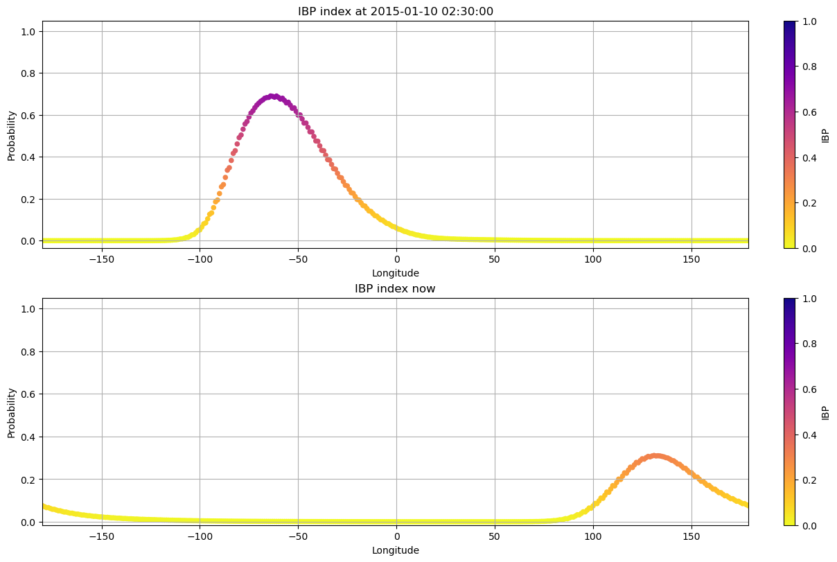
IBP index around the earth at specific time#
datum = datetime(2015, 1, 10, 2, 30).replace(tzinfo=timezone.utc)
# datum = datetime(2016, 4, 21, 22,50,0).replace(tzinfo=timezone.utc)

df1 = globalIBP(datum)
df2 = globalIBP(datetime.now())

fig, ax = plt.subplots(2, 1, figsize=(12, 8), layout="constrained")
df1.plot.scatter(
    x="Lon",
    y="IBP",
    title=f'IBP index at {datum.strftime("%Y-%m-%d %H:%M:%S")}',
    xlabel="Longitude",
    ylabel="Probability",
    grid=True,
    xlim=(-180, 179),
    c="IBP",
    colormap="plasma_r",
    vmin=0,
    vmax=1,
    ax=ax[0],
    sharex=False,
)
# sharex=False - must be there because there is still a bug and xlabel and tickmarks will not appear otherwise
df2.plot.scatter(
    x="Lon",
    y="IBP",
    title=f"IBP index now",
    xlabel="Longitude",
    ylabel="Probability",
    grid=True,
    xlim=(-180, 179),
    c="IBP",
    colormap="plasma_r",
    vmin=0,
    vmax=1,
    ax=ax[1],
    sharex=False,
)

for a in ax:
    a.set_ylim(top=1.05)

plt.show()
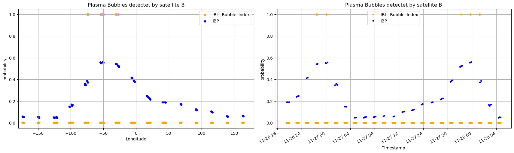
IBP Index along the orbit of a satellite#
starttime = datetime(2022, 11, 26, 17, 0, 0).replace(tzinfo=timezone.utc)
endtime = datetime(2022, 11, 28, 5, 0, 0).replace(tzinfo=timezone.utc)

sat = "B"

df = satelliteIBP(loadsatellitedata(starttime, endtime, sat))

display(df)

fig, axes = plt.subplots(1, 2, figsize=(17, 5), layout="constrained")

df.plot(
    x="Longitude",
    y="Bubble_Index",
    ax=axes[0],
    color="orange",
    kind="scatter",
    label="IBI - Bubble_Index",
)
# df.plot(x="Longitude", y="Bubble_Probability", ax=axes[0], color='g', kind='scatter', label='IBI - Bubble_Probability')
df.plot(x="Longitude", y="IBP", kind="scatter", ax=axes[0], color="b", label="IBP")

df.plot(
    y="Bubble_Index",
    ax=axes[1],
    color="orange",
    marker=".",
    linewidth=0,
    label="IBI - Bubble_Index",
)
# df.plot(x="Loy="Bubble_Probability", ax=axes[0], color='g', kind='scatter', label='IBI - Bubble_Probability')
df.plot(y="IBP", marker=".", linewidth=0, ax=axes[1], color="b", label="IBP")


axes[0].set_xlabel("Longitude")
axes[0].set_xlim(-180, 180)

for ax in axes:
    ax.set_ylabel("probability")
    ax.set_ylim(top=1.05)
    ax.legend()
    ax.set_title(f"Plasma Bubbles detectet by satellite {sat}")
    ax.grid()

plt.show()
| Longitude | Bubble_Probability | Flags_q | Spacecraft | Flags_Bubble | Radius | F107 | Flags_B | Latitude | Bubble_Index | Flags_F | IBP | |
|---|---|---|---|---|---|---|---|---|---|---|---|---|
| Timestamp | ||||||||||||
| 2022-11-26 17:32:38 | 41.735251 | 0.0 | 0 | B | 0 | 6888588.78 | 107.242806 | 0 | -44.990729 | 0 | 1 | NaN |
| 2022-11-26 17:32:39 | 41.736026 | 0.0 | 0 | B | 0 | 6888584.63 | 107.242790 | 0 | -44.927609 | 0 | 1 | NaN |
| 2022-11-26 17:32:40 | 41.736791 | 0.0 | 0 | B | 0 | 6888580.47 | 107.242774 | 0 | -44.864488 | 0 | 1 | NaN |
| 2022-11-26 17:32:41 | 41.737544 | 0.0 | 0 | B | 0 | 6888576.30 | 107.242758 | 0 | -44.801367 | 0 | 1 | NaN |
| 2022-11-26 17:32:42 | 41.738287 | 0.0 | 0 | B | 0 | 6888572.13 | 107.242742 | 0 | -44.738245 | 0 | 1 | NaN |
| ... | ... | ... | ... | ... | ... | ... | ... | ... | ... | ... | ... | ... |
| 2022-11-28 04:40:16 | -122.568657 | 0.0 | 0 | B | 0 | 6875021.45 | 107.127674 | 0 | 44.727242 | 0 | 1 | NaN |
| 2022-11-28 04:40:17 | -122.567896 | 0.0 | 0 | B | 0 | 6875010.38 | 107.127672 | 0 | 44.790612 | 0 | 1 | NaN |
| 2022-11-28 04:40:18 | -122.567125 | 0.0 | 0 | B | 0 | 6874999.32 | 107.127669 | 0 | 44.853982 | 0 | 1 | NaN |
| 2022-11-28 04:40:19 | -122.566342 | 0.0 | 0 | B | 0 | 6874988.26 | 107.127667 | 0 | 44.917352 | 0 | 1 | NaN |
| 2022-11-28 04:40:20 | -122.565549 | 0.0 | 0 | B | 0 | 6874977.22 | 107.127665 | 0 | 44.980722 | 0 | 1 | NaN |
32710 rows × 12 columns